This post consists of a few timeseries examples from my upcoming book on statistical and machine learning using Python, sequal to my co-authored book Python for SAS User
Parsing and Normalizing Dates
For most of the use cases we have encountered, pandas.to_datetime will parse date/time in string or number format to datetime format correctly.
However, when we want to be sure that parsing is done according to specification, we should provide directives, which are proceeded by the % sign. Just note that lower-case m represents month whereas upper caseM represents minute.
When using with apply, pd.to_datetime and datetime.strptime are equivalent, and they give the same results. One key difference is that pd.to_datetime can take a pandas series as an argument directly whereas datetime.strptime can only be used with apply.
After parsing, we can create new columns of date/time attributes for reporting or feature creation.
 df = pd.DataFrame({
'TimeStamp': ['2020/11/08 17:14:13', '2021/09/14 17:14:14', '2021/04/27 17:14:15']})

# all three methods give the same results
 df.TimeStamp.apply(lambda x: pd.to_datetime(x, format="%Y/%m/%d %H:%M:%S"))
 df.TimeStamp.apply(lambda x: datetime.strptime(x,"%Y/%m/%d %H:%M:%S"))
 pd.to_datetime(df.TimeStamp)
[Out]:
0   2020-11-08 17:14:13
1   2021-09-14 17:14:14
2   2021-04-27 17:14:15
Name: TimeStamp, dtype: datetime64[ns]

# handy function to add features
def parseDateCol(df, date_col):
	""" takes the date column and adds new columns with the features:
		yr, mon, day, day of week, day of year hour"""
	df['datetime'] = pd.to_datetime(df[date_col], format="%Y/%m/%d %H:%M:%S")
	df['year'] = df.datetime.dt.year
	df['month'] = df.datetime.dt.month
	df['mday'] = df.datetime.dt.day
	df['wday'] = df.datetime.dt.dayofweek
	df['yday'] = df.datetime.dt.dayofyear
	df['Hour'] = df.datetime.dt.hour
	#drop input column
	df = df.drop([date_col], axis = 1)
	return df
Out[122]:
             datetime  year  month  mday  wday  yday  Hour
0 2020-11-08 17:14:13  2020     11     8     6   313    17
1 2021-09-14 17:14:14  2021      9    14     1   257    17
2 2021-04-27 17:14:15  2021      4    27     1   117    17
Even when you run into a little more complicated situations, you can always chain apply with another apply to get the desired result.
 from datetime import datetime
 text = pd.Series(['something DEC2020','something DEC2021'])
 text.apply(lambda x: x[10:]).apply(lambda x: datetime.strptime(x,"%b%Y"))
Out[28]:
0   2020-12-01
1   2021-12-01
dtype: datetime64[ns]
To convert numbers to date/time, we can parse using directive, or first convert them to strings and then parse them to datetime.
 # numbers to datetime
 Time = 20210704
 pd.to_datetime(Time,format='%Y%m%d')
# or
 pd.to_datetime(str(Time))
[Out]: Timestamp('2021-07-04 00:00:00')

 Date = 70421
 pd.to_datetime(Date,format='%m%d%y').date()
Out: datetime.date(2021, 7, 4)
In financial reporting and financial risk modeling, it is common to aggregate and/or normalize data to quarterly.
# a very common format in financial reporting
 df = pd.DataFrame({'yq': ['2021Q1', '2021Q2', '2021Q3']})
 df['yq'] = pd.to_datetime(df.yq) +pd.offsets.QuarterEnd()
 print(df)
[Out]:
          yq
0 2021-03-31
1 2021-06-30
2 2021-09-30
Origin and Unit
Although pandas.to_datetime by default uses unix epoch origin, which is January 1, 1970, you can change it by providing your custom reference timestamp using the origin parameter. For example, for reading numbers that are representing SAS dates, we set origin=’1960-1-1’. In addition, unless a unit is provided, the default unit is nanoseconds, since that is how Timestamp objects are stored internally.
  pd.to_datetime(18081) #default unit in nanosecond
[Out]: Timestamp('1970-01-01 00:00:00.000018081')

  pd.to_datetime(18081, unit='D')
[Out]: Timestamp('2021-07-04 00:00:00')

# SAS default reference date
 pd.to_datetime(18081, unit='D',  origin='1960-1-1')
[Out]: Timestamp('2009-07-03 00:00:00')
# reverse operation
 (pd.to_datetime(18081, unit='D') - pd.Timestamp("1970-01-01")) // pd.Timedelta('1D')
[Out]: 18081
In case you want the parsed results to be a standard Python datetime object and not a pandas object, you can use dateutl.parser. Here is an example of using from parser from library dateutl to parse string into datetime object.
 from dateutil.parser import parse
 Time = "07/04/2021 19:00"
 parse(Time)
[Out]: datetime.datetime(2021, 7, 4, 19, 0)
For reference, see this ##table## for list of all the format codes that the C standard (1989 version) requires .
Normalizing Dates
When processing data, we would often need to normalize dates. This can be done using an appropriate offset.
For example, to normalize to end of quarter, do the following:
s1.index = s1.index + pd.offsets.QuarterEnd()
Alternatively, we can convert DatetimeIndex to PeriodIndex by the .to_period() function. The original dates will be normalized to period time spans. We can keep using the PeriodIndex or converted to DatetimeIndexusing either pd.to_timestamp or .astype(‘datetime64[ns]’). These operations can be useful for normalizing dates.
Example: CCAR Stress Testing Macroeconomic Variable
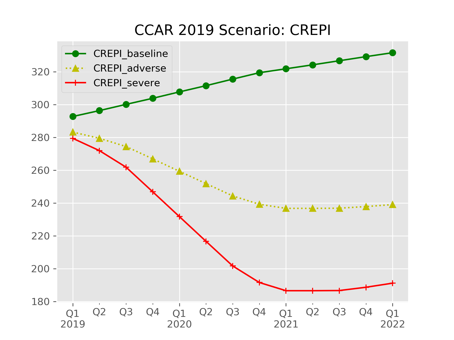
In this short example that encountered from work, we import zip file, extract, manipulate, and plot CCAR 2019 Federal Reserve Macro Scenarios

 from io import BytesIO
 from zipfile import ZipFile
 import pandas
 import requests
 content = requests.get(r"https://www.federalreserve.gov/supervisionreg/files/2019-macro-scenario-tables.zip")
 zf = ZipFile(BytesIO(content.content))
 for item in zf.namelist():
     print(item)
[Out]:
Table_2A_Supervisory_Baseline_Domestic.csv
Table_2B_Supervisory_Baseline_International.csv
Table_3A_Supervisory_Adverse_Domestic.csv
Table_3B_Supervisory_Adverse_International.csv
Table_4A_Supervisory_Severely_Adverse_Domestic.csv
Table_4B_Supervisory_Severely_Adverse_International.csv

 cols= ['Date','House Price Index (Level)','Commercial Real Estate Price Index (Level)']
 name_change = {'House Price Index (Level)':'HPI','Commercial Real Estate Price Index (Level)':'CREPI'}

 def ScenarioData(df, sffx):
     df.rename(columns=name_change, inplace=True)
     df[['year','qtr']]=df.Date.str.split("Q",expand=True)
     df.loc[:,'year']=df.year.astype('int')
     df.loc[:,'qtr']=df.qtr.astype('int')
     df['month'] = df.qtr*3
     df['day']= 1
     df.index = pd.to_datetime(df.loc[:,['year','month','day']])
     df.drop(['year','month','day','Date','qtr'], axis=1,inplace=True)
     df = df.add_suffix('_%s' %sffx)
     return df

 baseline = pd.read_csv(zf.open("Table_2A_Supervisory_Baseline_Domestic.csv"), usecols=cols)
 baseline =ScenarioData(baseline, "baseline")

 adverse = pd.read_csv(zf.open("Table_3A_Supervisory_Adverse_Domestic.csv"), usecols=cols)
 adverse = ScenarioData(adverse, "adverse")

 severe= pd.read_csv(zf.open("Table_4A_Supervisory_Severely_Adverse_Domestic.csv"), usecols=cols)
 severe = ScenarioData(severe,"severe")

 names = [baseline, adverse,severe]
 all_scenarios = pd.concat(names, axis=1)

 all_scenarios.filter(regex="CREPI").plot(style=['go-','y^:','r+-'],  title="CCAR 2019 Scenario: CREPI")
 plt.savefig(r"C:\Users\sache\OneDrive\Documents\python_SAS\Python-for-SAS-Users\Volume2\TimeSeries\images\CCAR Scenarios", dpi=300)
 plt.show()
Now we have covered construction of date and time objects, let us move on to the common types of time series operations: shifting, rolling, expanding, and aggregating in the coming sections.