In many business contexts, models not only need to be reasonable accurate but also must be interpretable and intuitive.
Linear models are sometimes preferred to more complex models, or at the minimum used as benchmark, for its strength in interpretability and reasonable performance.
In fact, linear regression is at the core of machine learning model interpretability.
There are many variations of linear regression models: ordinary least squares (aka “OLS”) linear regression, weighted least square regression, regularized OLS linear regression fitted by minimizing a penalized version of the least squares cost function, generalized linear model, or are solved by gradient descent, and so on.
It is important to distinguish linear regression and the least squares approach. Although the terms “least squares” and “linear model” are closely linked, they are not synonymous.
- Linear models predict averages, and they refer to model specification being a weighted sum of the parameters for a continuous target variable such as y = a + bx.
- Whereas least squares refers to how the loss function is defined. Least squares is a way of defining the objective function of a model, which refers to the c00ore of the problem that models are trying the solve: to have the least amount of errors in making predictions. You can define errors in different ways: sum of absolute error, sum of square of error, weighted errors, or other definitions.
Simple example
We will start with the simplest one-feature dataset, the Anscomebe quartet dataset. We use the seaborn library to plot the four stylized subsets of Anscomebe.
import seaborn as sns
anscombe = sns.load_dataset("anscombe")
sns.lmplot(x="x", y="y", col="dataset", hue="dataset", data= anscombe, palette="muted", scatter_kws={"s": 50, "alpha": 1})
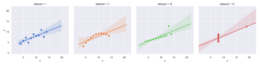
Note: The data was constructed in 1973 by Frank Anscombe (13 May 1918 – 17 October 2001), an English statistician, who had stressed that "a computer should make both calculations and graphs". He illustrated the importance of visualizing data with four data sets now known as Anscombe's quartet. Frank Anscombe was brother-in-law to John Tukey.
The four subsets, each with 11 data points, have distinct characteristics despite almost identical statistics in count, mean, median, standard deviation, and Pearson correlation between x and y. If you fit OLS linear regression on them, you get the same intercept, coefficient, and same p-values of 0.022 for each of them.
- The first set of data appears to be the typical linear relationship and follow the assumption of normality.
- The second set of data does not seem normally distributed. A quadratic line would be a better fit.
- The third set of data has perfect linear relationship between x and y, but is affected by one outlier. Unless the outlier is important to keep, one should consider robust regression.
- The fourth set of data does not show any linear relationship between x and y, even though the Pearson linear correlation is large.
| x_I | y_I | x_II | y_II | x_III | y_III | x_IV | y_IV | |
|---|---|---|---|---|---|---|---|---|
| 0 | 10 | 8.04 | 10 | 9.14 | 10 | 7.46 | 8 | 6.58 |
| 1 | 8 | 6.95 | 8 | 8.14 | 8 | 6.77 | 8 | 5.76 |
| 2 | 13 | 7.58 | 13 | 8.74 | 13 | 12.74 | 8 | 7.71 |
| 3 | 9 | 8.81 | 9 | 8.77 | 9 | 7.11 | 8 | 8.84 |
| 4 | 11 | 8.33 | 11 | 9.26 | 11 | 7.81 | 8 | 8.47 |
| 5 | 14 | 9.96 | 14 | 8.1 | 14 | 8.84 | 8 | 7.04 |
| 6 | 6 | 7.24 | 6 | 6.13 | 6 | 6.08 | 8 | 5.25 |
| 7 | 4 | 4.26 | 4 | 3.1 | 4 | 5.39 | 19 | 12.5 |
| 8 | 12 | 10.84 | 12 | 9.13 | 12 | 8.15 | 8 | 5.56 |
| 9 | 7 | 4.82 | 7 | 7.26 | 7 | 6.42 | 8 | 7.91 |
| 10 | 5 | 5.68 | 5 | 4.74 | 5 | 5.73 | 8 | 6.89 |
OLS from Scratch
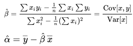
The OLS in one variable can be solved in linear algebra, or beginning calculus, or, with a few more steps, even middle school algebra.
def ols(x, y):
  n = np.size(df.y)
  m_x = np.mean(df.x)
  m_y = np.mean(df.y)
  xy = np.sum((df.x - m_x)*(df.y - m_y))
  xx = np.sum((df.x - m_x)**2)
  b1 = xy/xx
  b0 = m_y - b1*m_x
  print("dataset %s" %i)
  print("intercept:  {0:0.3f}".format(b0))
  print("coefficient: {0:0.3f} \n".format(b1))
for i in ['I','II','III', 'IV']:
  df = anscombe[anscombe.dataset=='%s' %i]
  ols(df.x, df.y)
#  Out:
#  dataset I
# intercept:  3.000
# coefficient: 0.500

# dataset II
# intercept:  3.001
# coefficient: 0.500

# dataset III
# intercept:  3.002
# coefficient: 0.500

# dataset IV
# intercept:  3.002
# coefficient: 0.500
OLS from sklearn
The sklearn.LinearRegression class is a wrapper around the lstsq function from scipy.linalg.
LinearRegression(copy_X=True, fit_intercept=True, n_jobs=None, normalize=False)
It is quite basic, with basically two options other than copy_X and n_jobs.
The two options are intuitive if we understand the formula for the solution of weights in OLS loss function:
- fit_intercept: bool, optional, default True. Whether to calculate the intercept for this model. If set to False, no intercept will be used in calculations (i.e. data is assumed to be centered already, in other words, the mean of the data is subtracted from each data point). Visually, the fitted line will pass through the origin, if set to False.
- normalize: bool, optional, default False. This parameter is ignored when fit_intercept is set to False. If True, the regressors X will be normalized before regression by subtracting the mean and dividing by the l2-norm. If we wish to standardize, please use sklearn.preprocessing.StandardScaler before calling fit on an estimator with normalize=False.
from sklearn.linear_model import LinearRegression
from sklearn.metrics import mean_squared_error, r2_score
X =df.x.values.reshape(-1,1) #reshape to 2-dimensional
y =df.y.values
# instantiate the LinearRegression object and fit data
model = LinearRegression()
model.fit(X, y)
# model parameters
print('Coefficient(s): ', (*['{0:0.3f}'.format(i) for i in model.coef_]),sep='\n' ) # using separator would be convenient when
print('Intercept:{0:0.3f}'.format(model.intercept_))
# model predictions
y_pred = model.predict(X)
print("Mean squared error: %.2f"
      % mean_squared_error(y, y_pred))
print('R square: %.2f' % r2_score(y, y_pred))
alpha=0.8
title ='OLS Regression for Anscomebe Dataset 1'
f, ax =plt.subplots(1, 1)
plt.rcParams["figure.figsize"] = (5,5)
ax.plot(X, y,  alpha=alpha, linestyle='None', marker='o')
ax.text(4,10, r'$R^2$=%.2f MSE=%.2f' % (r2_score(y, y_pred) ,mean_squared_error(y, y_pred)))
ax.text(4,8.5, 'Intercept:   {0:0.2f}'.format(model.intercept_))
ax.text(4,9,   'Coefficient:{0:0.2f}'.format(model.coef_[0]))
ax.plot(X, y_pred, alpha=alpha)
ax.set_title('%s' %title)
ax.set_ylabel('y')
ax.set_xlabel('X')
plt.savefig("images/%s.png"%title,dpi=300, tight_layout=True)
plt.clf()
plt.close()
# Out:
# Coefficient(s):
# 0.500
# Intercept:3.000
# Mean squared error: 1.25
# R square: 0.67

- When requesting R square using
r2_score, the order matters. It should be r2_score(y_actual, y_pred). The actual value goes first, then the predicted. We will get a wrong result if the order is not followed. - In case we did not know it already, the square of the pearson correlation coefficient is R square for the one-feature case. So next time if we have doubts about which implementation of OLS, sklearn or statsmodel, is correct, this could be one of your testing tools.
OLS Using Statsmodels
To get p-values and other statistical metrics like those from SAS and R, we use the Python statsmodels library.
import statsmodels.formula.api as smf
df = anscombe.loc[anscombe.dataset=='I',['x','y']]
smod = smf.ols(formula ='y~ x', data=df)
result = smod.fit()
print(result.summary())
For plain OLS, we recommend we use statsmodels.formula.api instead of statsmodels.api, even though their names sound similar. The formula api uses the patsy package to convert data and formula into matrices. The latter requires adding a column of constants to the array of independent variables commonly denoted as “X”.
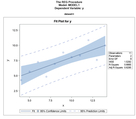
OLS Using SAS
SAS is the king of statistical analysis without much code. SAS REG procedure is a general-purpose procedure for regression.
It provides the following with very little coding.
- multiple model statements
- nine model-selection methods: default (full model), forward, backward, stepwise, maxr (forward selection to fit the best one-variable model, the best two-variable model, and so on), minr, rsquare (finds a specified number of models with the highest r square in a ange of model sizes), adjrsq (finds a specified number of models with the highest adjusted r square in a range of model sizes), and CP
- interactive changes both in the model and the data used to fit the model
- linear equality restrictions on parameters
- tests of linear hypotheses and multivariate hypotheses
- collinearity diagnostics
- predicted values, residuals, studentized residuals, confidence limits, and influence statistics
- correlation
- requested statistics available for output through output data sets
- plots
It outputs tons of information for just a few lines of code.
PROC REG DATA = df (WHERE=(dataset='I'));
MODEL y=x;
RUN;

Diagnostics are important too!
The outputs show that the model is the right type of model for this data, and that the parameter coeffcient is trustworthy. For new data coming from the same population, we can apply this model with confidence.

If we add just one line of code BY dataset;, we get the OLS for each of the Anscombe quartet. There are many other options too.
Other SAS/STAT procedures that perform at least one type of regression analysis are the CATMOD, GENMOD, GLM, LOGISTIC, MIXED, NLIN, ORTHOREG, PROBIT, RSREG, and TRANSREG procedures. SAS/ETS procedures are specialized for applications in time series or simultaneous systems.
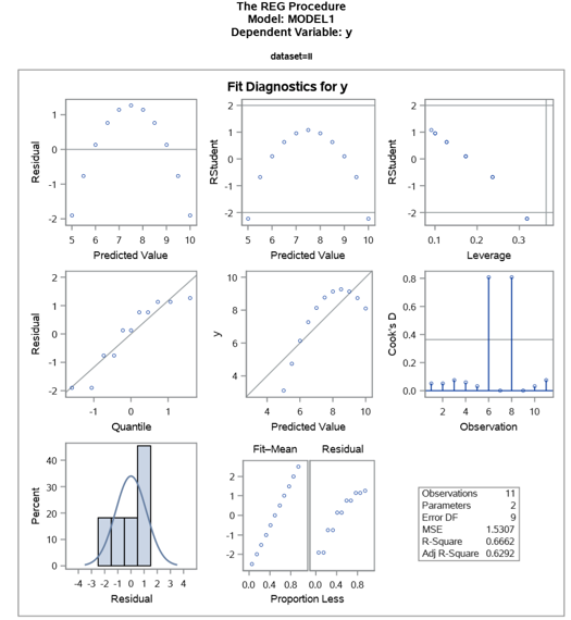
Less perfect case
We will apply the same algorithm to the second subset of the Anscombe quartet. The code is exactly the same.
As noted in the introduction, the subsets have identical statistics in count, mean, median, standard deviation, and Pearson correlation between x and y.
Because it has same intercept, same coefficient, and even the p-values of 0.022, many would have thought this was the perfect model. But this is probably not the right model for this data, which we could tell by looking at the data at the onset, or by examining the residual diagnostics as shown in SAS output below.
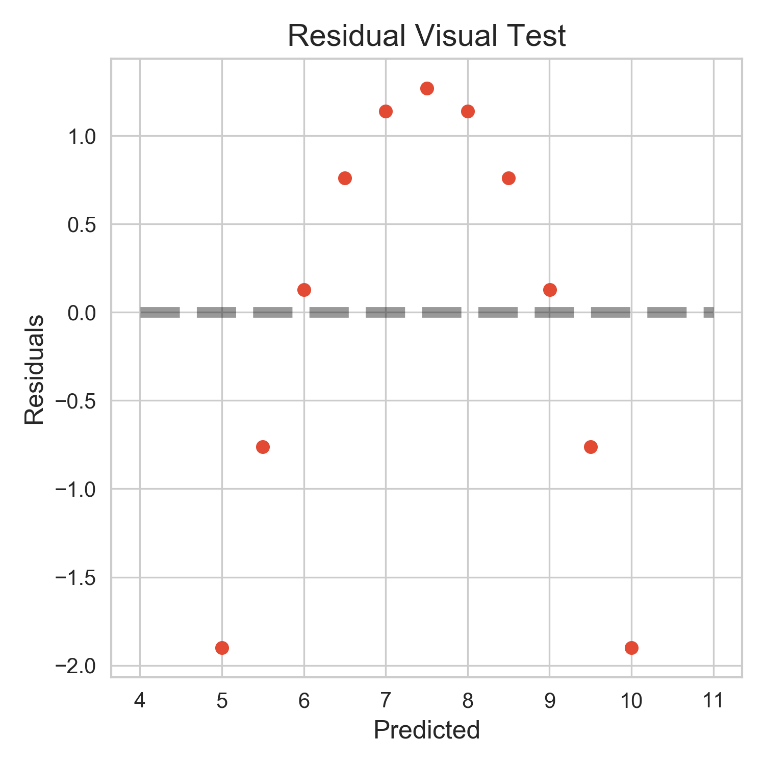
The residual plot shows that the OLS assumptions do not stand. From the figure below, we see that the residule plot looks like a parabola and does not look anyway close to random along the predicted, which does not support assumptions of OLS: linear relationship, homoscedasticity, and independence.
Without diagnostics or visual analysis of the data, it would have been hard to tell any potential problems if we look at statistics and performance scores only.
We should probably transform the variable, for example, using power transform (note that y = a + bx^2 is still linear regression)
df = anscombe.loc[anscombe.dataset=='II',['x','y']]\
.copy()
X =df.x.values.reshape(-1,1)
y =df.y.values
model = LinearRegression()
model.fit(X, y)
y_pred = model.predict(X)

def residual_visual_test(y, y_pred):
    resid = y - y_pred
    fig, ax = plt.subplots(1,1)
    ax.scatter(y_pred, resid)
    ax.set_title('Residuals vs. Predicted Values')
    ax.set(xlabel='Predicted', ylabel='Residuals')
    ax.plot([min(y_pred)-1, max(y_pred)+1],[0,0],'--k',lw=5,alpha=0.4)
    plt.savefig(r"./images/Residual Visual Test.png", dpi=300)

residual_visual_test(y, y_pred)
More
OLS is old and fundamental. Its coefficients can be summarized as a dot product normalized by the vector space of the input features.
To do it correctly, the assumptions should not be too far off. Checking the fit diagnostics is a way to see if the assumptions are met.
If the assumptions are far from true, we have many other ways besides basic OLS.