Century old t-tests formulated to ensure beer quality was formally adopted in statistics and, now, AB testing

The t-test was developed in early 1900s as an economical (small samples) way to check for differences in mean quality of batches of Guinness beer that were small in sample sizes. William Gosset , the Head Brewer of Guinness and pioneer of modern statistics empirically, by trial and error, found a formula for a t-distributed random variable.
Gosset was a friend of both Karl Pearson and Ronald Fisher.
It is called the t-test because the test statistics is from a t distribution, which tends to the z (normal) distribution when n is large (when n>30, they are almost identical).
As William Gosset noted in his original publication The Probable Error of a Mean, while it is applicable to samples from population that are normally distributed, “the deviation from “normality must be very extreme to lead to serious error.”
Why did he and others focus on population that are normal distributed as opposed to a different kind of distribution? I guess that’s partially due to computational limitations.
Normal distribution tables and calculus were the best technology at that time.
The t-test is a type of signal-to-noise test.
One-sample t-test of the mean
Also called the “location test”, the one-sample t-test compares one sample mean to a null hypothesized mean.
The comparison has to be standardized by something–the standard error the mean (population standard deviation, approximated by sample, devided by square root of sample size)
The t-statistics is more or less defined as followed:
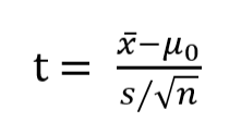
The one-sample t-statistics can be interpreted as the signal-to-noise ratio, where the numerator is signal (aka “effect size”) and the denominator (standard error of the mean) the noise.
The larger the numerator, the higher the signal. The higher the variance, the lower the signal to noise ratio. The signal must be large enough to stand out from the noise for the test result to be significant.
Paired t-test
A paired t-test Is just a one-sample t-tests as the difference between paired observations (e.g., before and after) is the test data with null hypothesis that the mean is 0 (i.e. no difference).
To determine that the groups are different, the t-value needs to be large enough.
Two-sample (unpaired) t-test
Unpaired-samples: aka “independent-samples”, “between samples” test if two different groups have the same mean. In a 2-sample t-test, the denominator is still the noise. We can either assume that the variability in both groups is equal or not equal. Either way, the principle remains the same: we are comparing signal to noise.
Just like with the 1-sample t-test, for any given difference in the numerator, as we increase the noise value in the denominator, the t-value becomes smaller.
To determine that the groups are different, we need a t-value that is large enough.
For details, see NIST Two-Sample t-Test for Equal Means
Note: T statistics is equivalent to F statistics when there are only two populations/categories.
critical value
A quick review of t-test and critical values is in example below. The ppf function scipy.stats gives the the ‘quantile’, which is the critical value for the probability and degree of freedom we specify.
from scipy import stats
print('{0:0.3f}'.format(stats.t.ppf(1-0.025, loc=0, scale=1, df=1)))
# 12.706
print('{0:0.3f}'.format(stats.t.ppf(1-0.025, loc=0, scale=1, df=9)))
# 2.262
print('{0:0.3f}'.format(stats.t.ppf(1-0.025, loc=0, scale=1, df=999)))
# 1.962
print('{0:0.3f}'.format(stats.norm.ppf(1-0.025, loc=0, scale=1)))
# 1.960
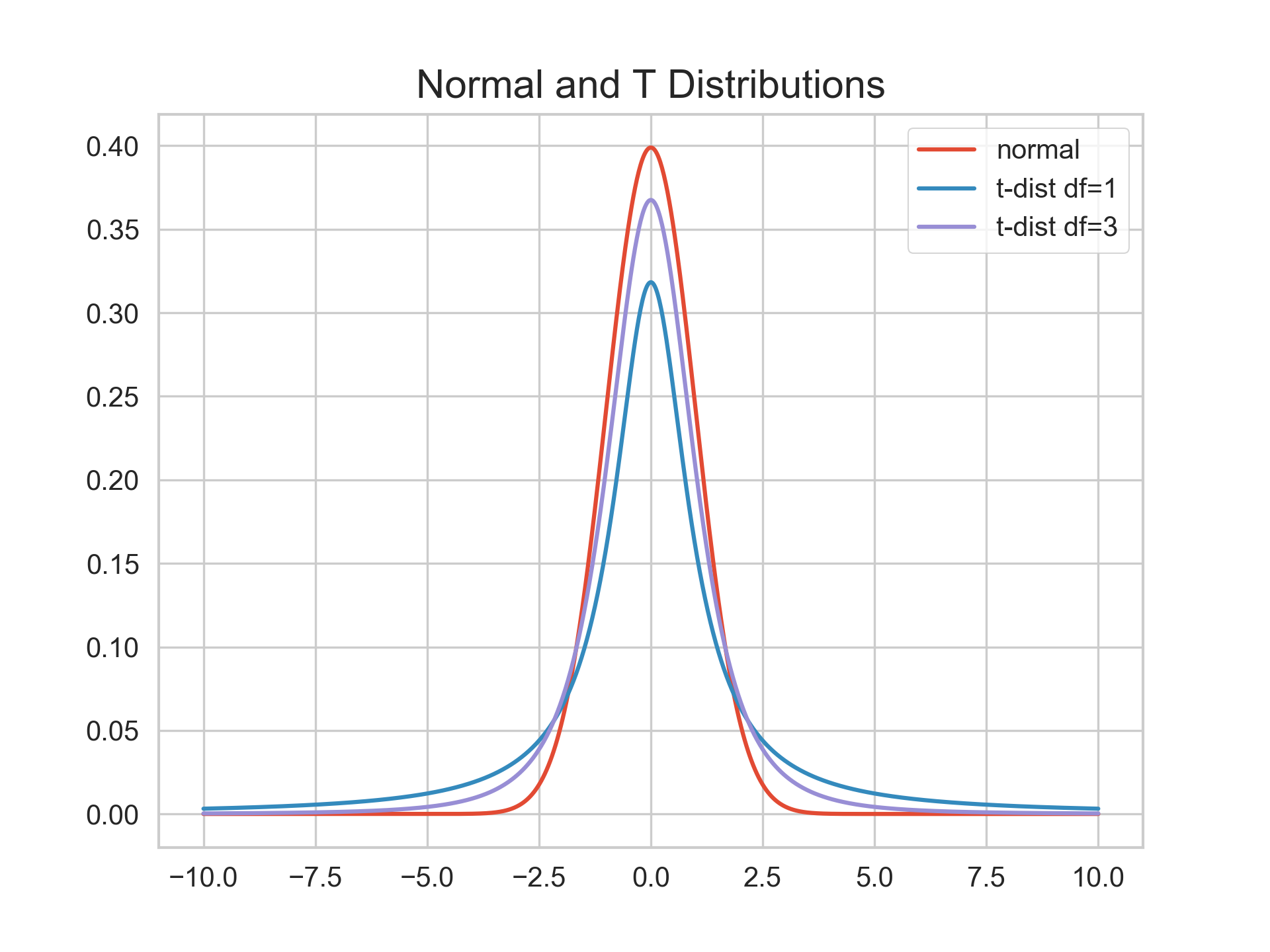
To roughly explain the differences in the critical values in the example above for various degrees of freedom, please see the plot below. The smaller the degrees of freedom, the probability density curve is more stretched to the two tails. The larger the degrees of freedom, the closer it is to the normal distribution.
from scipy import stats
# plot normal Sarah
import numpy as np
import scipy
import pandas as pd
from scipy.stats import norm
import matplotlib.pyplot as plt
n =1000
bins = np.linspace(-10, 10, n)
fig, ax = plt.subplots()
plt.plot(bins,stats.norm.pdf(bins),label='normal')
plt.plot(bins, stats.t.pdf(bins, loc=0,scale=1,df=1), label='t-dist df=1')
plt.plot(bins, stats.t.pdf(bins, loc=0,scale=1,df=3), label='t-dist df=3')
plt.legend()
plt.title("Normal and T Distributions")
plt.savefig("Normal_T_Distribution",dpi=300)
plt.show()
Limitations of t-tests:
- Sample and population should not be too skewed in distribution (i.e. very roughly normal)
- Each group should have about the same number of data points. Comparing large and small groups together may give inaccurate results.
Overcoming limitations:
- Simulations or shuffling
- Non-parametric tests, like the Mann-Whitney rank test can work with non-normal distributions and ordered-level data. On the other hand, these tests are also less powerful.
AB tests
Does mathematics need new clothes?
No. Only people do.
T tests and other statistical tests have been “re-branded” in Silicon Valley as “AB” test.