There is a trade off between accuracy and interpretability. High accuracy models have low interpretability and potential problems. Explainable AI (XAI) is to have your cake and eat it too.

In linear regression, there has been well-established theory and diagnostics on how a model works, such as the model statement y = a + bX, confidence interval, p-value (assuming x is not relevant what’s the chance of having this kind of relationship to y) and etc.
In linear regression and situations where linear regression are used (in neural network as well) balance of bias and variance can be strived for by using regularizers (for penalizing more variables and/or shrinking weights) to prevent overfitting and instability due to multicollinearity.
So, yes, machine learning is powerful leveraging computing power and data. But then, why should anyone just accept black boxes and expect less from the ML/AI models? Some questions that may puzzle ML folks are questions from senior executives “what are the degrees of freedom of this model?”
For low-consequence machine learning models or those that we find to be the best option such as those used in postal code sorting, image recognition, explanation is not necessary as long as we know that the algorithms are working as demonstrated–Blackboxes are fine.
However, in many context, especially those with high stake especially involving people, such as health care/medicine, financial industry, and the military, to be able to interprete model output is as important as the model.
In regulated industries, interpretability is required before adoption. Therefore, interpretability is essential, as it was important to evaluate confidence interval and p-values in traditional statics.
In addition, bias prevention is important not only for regulatory and fairness concerns but also for more` accurate predictions.
A genearal introduction from theoretical point of view on definitions of interpretability is in Towards A Rigorous Science of Interpretable Machine Learning.
Interpretable AI (XAI) has been a very active area in recent years, motivated by commercial reasons (to gain from the available technology) and regulatory needs. For example, the House Financial Services Committee expert hearing 02/12/2010 :Task Force on Artificial Intelligence: Equitable Algorithms” discussed definitions of fairness, Dr. Philip Thomas proposed Seldonian framework altorithm. The word “Seldonian” refers to Hari Seldon, a finctional character by Isaac Asimov, who claimed three laws of robotics beginning with the injunction that “A robot may not injure a human being or, through inaction, allow a human being to come to harm.”
There are two categories of tools in both the old and latest machine learning interpretability methods and models:
- tools for helping us to understand ML/AI models: PDP, ICE, Tree Interpreter (linear representation) LIME (Linear regression locally).
- monotonicity as regularizers to ensure interpretability built into the models.
Here is a quick summary of some of the old and new XAI methods and algorithms:
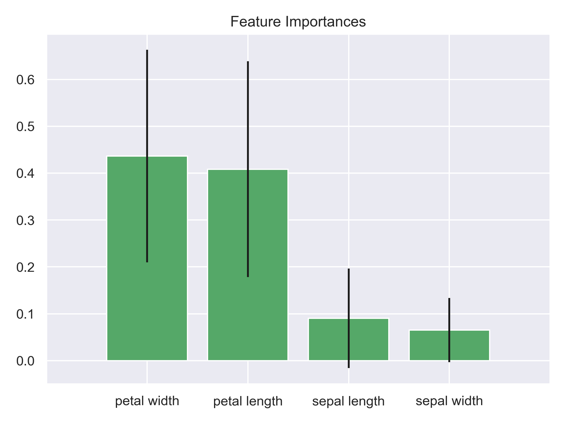
Variable Importance and Plot
Mostly suitable for tree based models, using gini importance or entropy as the metric for measuring difference due to variables at each split of trees. But it does not explain which variables impact the predictions for a particular variable and how.
from sklearn.ensemble import ExtraTreesClassifier
from sklearn.datasets import load_iris
iris = load_iris()
X = iris.data
y = iris.target

forest = ExtraTreesClassifier(n_estimators=250,
                              random_state=0)

forest.fit(X, y)
importances = forest.feature_importances_
feature_names = [i.split(' (', 1)[0] for i in iris.feature_names]

stdev = np.std([tree.feature_importances_ for tree in forest.estimators_],
             axis=0)

importances_df= pd.DataFrame(zip(importances, stdev), columns=['importance','stdev'], index=feature_names)
importances_df.sort_values(by='importance',ascending=False, inplace=True)
# Print the feature ranking
print("Feature ranking:")
print(importances_df)

# Plot the feature importances of the forest
plt.figure()
plt.title("Feature importances")
plt.bar(range(X.shape[1]), importances_df.importance,
       color="g", yerr=importances_df.stdev, align="center")
plt.xticks(range(X.shape[1]), importances_df.index)
plt.xlim([-1, X.shape[1]])
plt.tight_layout()
plt.show()
A side note: A Comparison of R, SAS, and Python Implementations of Random Forests documented comparisons on different variable importance implementation amongst Python R SAS on one dataset.
Tree Interpreter
Tree Interpreter (formulated by Andos Saabas) is an ingenius method to understand feature contribution in trees using linear regression representation.
Since a forest is nothing but a collection of trees (average of the scores from trees), if we can explain a tree, we can explain a forest.
Since a tree is nothing but the growth from root to leaves, if we can explain each split/step, we can explain a tree.
In this formulation, bias corresponds to the intercept in linear regression while “contribution” of a variable is somewhat similar to beta*x.
It is intuitive and beautiful. One ‘limitation’ is that for joint contributions cases such as XOR you will need to explicitly test the joint contribution.
from sklearn.ensemble import RandomForestClassifier
from treeinterpreter import treeinterpreter as ti
import numpy as np
from sklearn.datasets import load_iris
iris = load_iris()
X = iris.data
y = iris.target
rf = RandomForestClassifier(max_depth = 4)
idx = np.arange(len(iris.target))
np.random.shuffle(idx) #inplace

rf.fit(iris.data[idx][:100], iris.target[idx][:100])
# predict for a single instance.
instance = iris.data[idx][100:101]
print (rf.predict_proba(instance))

# Breakdown of feature contributions:
prediction, bias, contributions = ti.predict(rf, instance)
print( "Prediction", prediction)
print( "Bias (trainset prior)", bias)
print( "Feature contributions:")
for c, feature in zip(contributions[0],
                             iris.feature_names):
    print( feature, c)
Partial dependence plot (PDP)
Kind of like partial derivative, but the key difference is on predicted instead of actual. So it tells one-dimensionally how the model predictions reacts to changes to one single variable. At each value of a variable in question, the model is evaluated for all observations of the other model inputs, and the predictions are then averaged.
In general, the steeper the slope, the more important the variable. Just pay attention and make sure the the plots are on the same axis if you are comparing slope.
But, the relationship they depict is only valid if the variable of interest does not interact strongly with other model inputs.
In other words, PDPs can be misleading if there are divergent behavior caused by interactions as it is looking at the average of model response.
As an example, we plot the top sixe most important features according to a random forest model on the Boston Housing dataset using the convinient plot_partial_dependence method from sklearn.
from sklearn.inspection import plot_partial_dependence
plt.style.use('ggplot')
fig, ax = plt.subplots(2, 3, figsize=(12,5))
plt.tight_layout()
plot_partial_dependence(rfc, X, feat_imp.nlargest(6).index, n_cols=3, ax=ax)
Note that even in this super clean dataset, the PD plots do not show monotonicity between modeled housing price and the features. If we dig a bit deeper (such as using 2D PD or ICE), we will observe interactions.
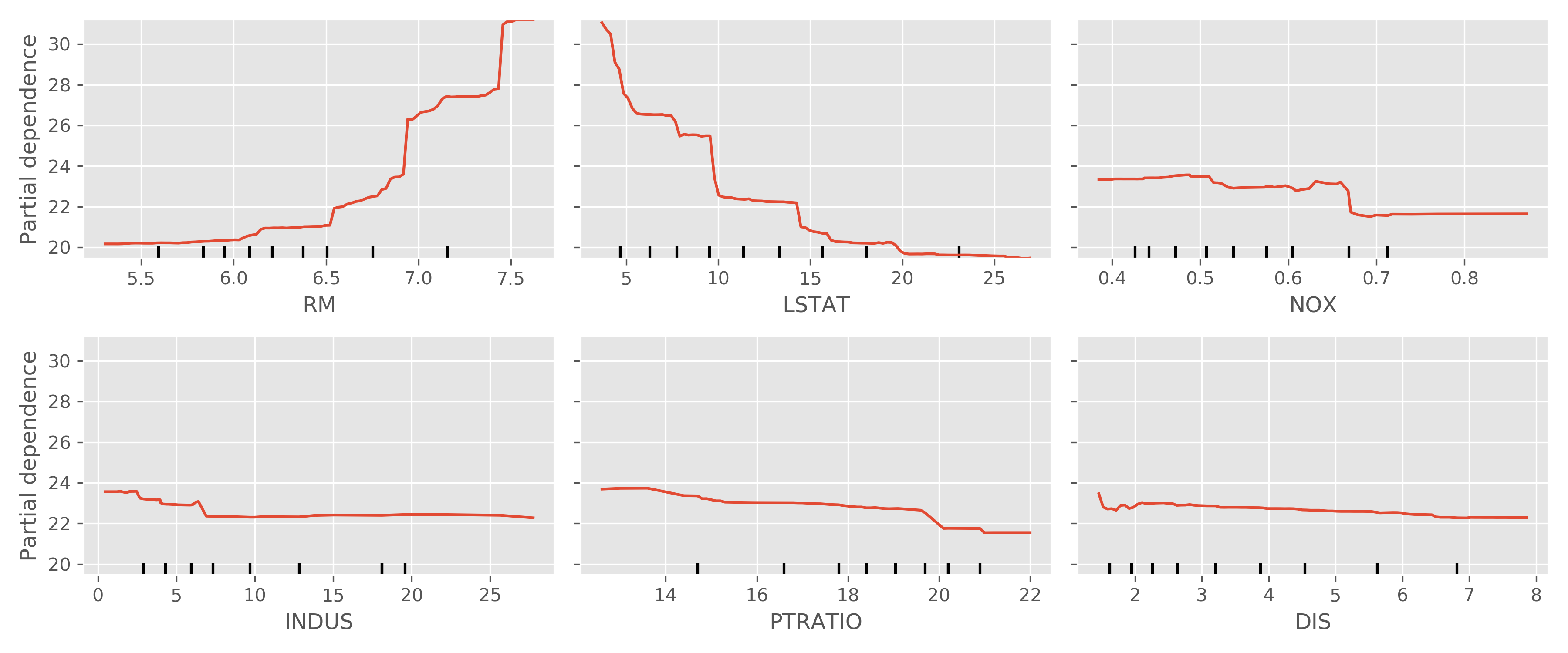
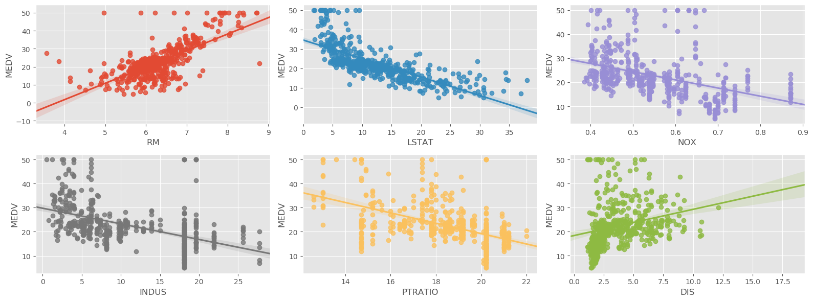
Comparing them with scatterplots of the same six features with target,while there are similarities observed between the subplots of the PDPs, they are far from the same:
- scatterplot: is at obervation level between predictor and target
- PD plot: is between predictor and average prediction
But you kind of can imagine that PDP is approximating collapsing target along the y-axis in a scatterplot.
Note that had we used a linear regression model, the direction of ‘DIS’ (distance to employment ceters) would have been unintuitive.
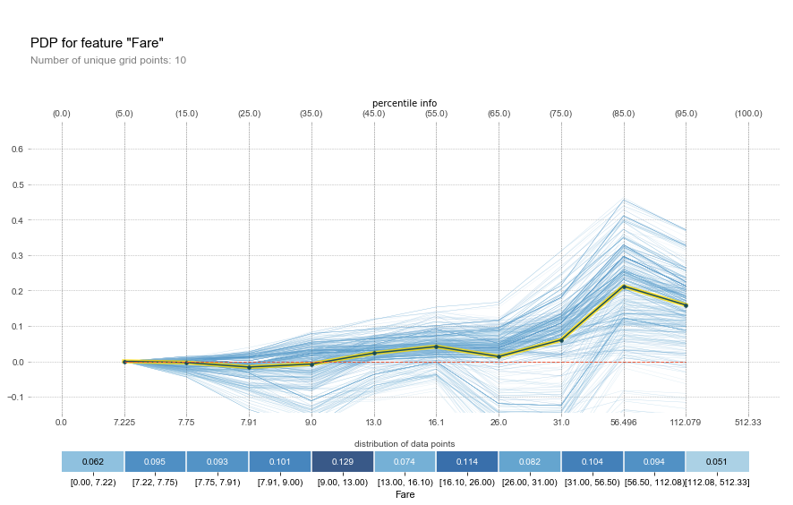
Individual conditional expectation plot (ICE)
Individual conditional expectation plots were introduced in in “Peeking Inside the Black Box: Visualizing Statistical Learning with Plots of Individual Conditional Expectation” (arXiv:1309.6392).
Like PD, ICE is another model agnostic method to help us interprete models.
As its name implies, it plots at individual observation level. In ICE plots the predictions are not aggregated, i.e., the plot is at observation level, over the range of X values of the variable of interest.
ICE plots can help us see individual differences and identify subgroups and interactions between model inputs.
Since ICE is at observation level, it quickly becomes a scaling issue. So in practice, we often bin the variable in question.
An example from Python PDPbox
LIME
Abbreviated for “Local Interpretable Model-Agnostic Explanations”. It was formulated first by Marco Tulio Ribeiro and others in 2016.
It is model agnostic and can be applied to most models by creating localized linear regression model around a particular observation based on a perturbed sample set of data, which is based on the distribution of the original input data.
The sample set is scored by the original model and sample observations are weighted based on distance to the observation of interest.
Next, variable selection is performed using the L1 LASSO technique as in linear models.
Finally, a linear regression is created to explain the relationship between the perturbed input data and the perturbed target variable.
The final result is an easily interpreted linear regression model that is valid near the observation of interest.
This is available from the library lime.
Shapley Values
Mostly suitable for tree based models, and found to be relatively acurate in approximating the decision attributes.
It is included in Python library XGBoost, and separately in the shap library. It was formularized by University of Washington researcher Scott Lundberg (currently senior researcher at Microsoft).
This is available from the library shap. See here.
import xgboost
import shap

# load JS visualization code to notebook
shap.initjs()

# train XGBoost model
X,y = shap.datasets.boston()
model = xgboost.train({"learning_rate": 0.01}, xgboost.DMatrix(X, label=y), 100)

# explain the model's predictions using SHAP
# (same syntax works for LightGBM, CatBoost, scikit-learn and spark models)
explainer = shap.TreeExplainer(model)
shap_values = explainer.shap_values(X)

# visualize the first prediction's explanation (use matplotlib=True to avoid Javascript)
shap.force_plot(explainer.expected_value, shap_values[0,:], X.iloc[0,:])
TensorFlow Lattice
Essentially interpolated look-up tables, TensorFlow Lattice is a library that implements constrained and interpretable lattice based models. It is an implementation of Monotonic Calibrated Interpolated Look-Up Tables in TensorFlow.
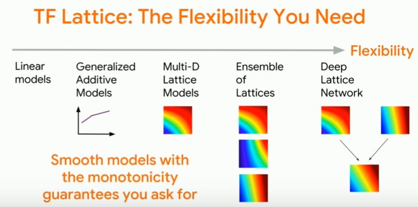
The library enables you to inject domain knowledge into the learning process through common-sense or policy-driven shape constraints.
For an overview, see Google scientist Maya Gupta’s TensorFlow Dev Summit 2019 video TF Lattice: Control Your ML with Monotonicity.
Here are a few screenshots from the video.
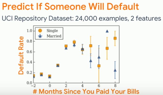
Tree-based machine learning models and neural networks can have high accuarcy, but can be prone to fitting into random noises in the data (even with cross validation), which do not make sense, and can possibly be unethical.
Often, how we combat “overfitting” related problems is by regularization.
But any regularization technique will hurt the model accuracy and cannot guarantee solving the problem.
TF Lattice hits the problem exactly by using monotonicity as the regularizer.
1-d lattice is just a piecewise linear function.
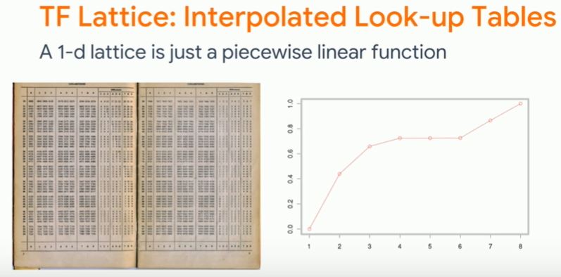
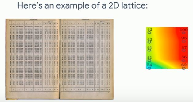
Multidimensional lattice are trained using empirical risk minimization, the same as you see with DNN.
Recommended resources:
Confidence intervals
The same resampling techniques that make ensemble models so successful can be used to compile confidence intervals, and generate similar concepts like p-values.
More
Back to the start, why we should accept less in powerful machine learning!
If we have insufficient or poor data, or omit important variables, no magic will compensate. Like in linear regression models, machine learning cannot make something out of nothing, which we should try to ensure via explainability.
As Rep. Loudermilk questioned in the hearing 02/12/2010 :Task Force on Artificial Intelligence: Equitable Algorithms”: we, as human, are biased whereas algorithm is mathmatics. Are we going to focus on algorithm or the appropriateness of the data. If it is the appropriateness of the data, then have to prove that the data is wrong, not because of the biasness of ourselves”