This post consists of a few timeseries examples from my upcoming book on statistical and machine learning using Python, sequal to my co-authored book Python for SAS User
Compare rolling with resampling
Rolling window and resampling are two important time series processing methods.
The first key difference between them is whether frequency changes or not. Their second key difference is whether restrict to datetime indices.
In windowing, statistics are calculated from the windowed rows when “expanding” through each row and frequencies are not changed.
Whereas resampling changes frequencies of the data via up sampling (higher frequency) or down sampling (lower frequency). In other words, resampling will change the row number count. For example, when daily observations become monthly, the row count will be reduced by a factor of 1/12.
Resampling is time-based groupby and requires datetime index. Whereas, rolling window can be applied to any pandas object, not restricted to those with datetime indices.
Resampling and rolling can be used together. For example, the following code first sum data by day and then compute seven-day moving average:
df.resample("1d").sum().fillna(0).rolling(window=7, min_periods=1).mean()
Rolling Window Statistics
Rolling in pandas is implemented both as time-window and count-based, which produce different results when the index is irregular. This could be confusing if not understood properly.
What we mean by time-window is that the operation is faithful to time, not to observation count.
To avoid getting unexpected result, it is best to be explicit by specifying the parameters given the dual implementations for count-based window and time-based window.
There are two parameters for determining how the rolling statistics are computed:
window: the size of the window min_periods: the minimum number of observations in window required to have a value; For a window that is specified by an offset, min_periods will default to 1. Otherwise, min_periods will default to the size of the window.
Below compares count-based window and time-based window for regular (without gaps) date time index.
In the first example, because an integer is used for the window, rolling(2).sum() assumes that the min_periods equals to the window size. It returns what we expect: the first row is NaN because it has only 1 observation. The last two rows are NaN because summing with NaN returns NaN.
In the second example, we see that rolling(window = ‘2d’).sum() seems to have ignored the NaN. This behavior is because min_periods=1 is the default setting for offset window.
The third example gives the same result as Example 2 because of specified min_periods= 1 is specified. For regular dateimeIndex, to get the same results from count-based and time-based windows, remember to specify the same min_periods.
df = pd.DataFrame({'x': [0, 1, 2, np.nan, 4]},
                    index=pd.date_range('20210101',
                    periods=5, freq='d'))
df
[Out]:
              x
2021-01-01  0.0
2021-01-02  1.0
2021-01-03  2.0
2021-01-04  NaN
2021-01-05  4.0
# Example 1
df.rolling(window = 2).sum()
[Out]:
              x
2021-01-01  NaN
2021-01-02  1.0
2021-01-03  3.0
2021-01-04  NaN
2021-01-05  NaN
# Example 2
df.rolling(window = '2d').sum()
[Out]:
              x
2021-01-01  0.0
2021-01-02  1.0
2021-01-03  3.0
2021-01-04  2.0
2021-01-05  4.0
# Example 3
df.rolling(window=2, min_periods=1).sum()
Out[11]:
              x
2021-01-01  0.0
2021-01-02  1.0
2020-01-03  3.0
2020-01-04  2.0
2020-01-05  4.0
The next example makes the comparisons for irregular datetime index. Contrasting to an integer rolling window, offset window will have variable window length corresponding to the time. Again, the default for offset window min_periods is 1. To see why Example 1 and Example 2 have different results, it may be helpful to look at Example 3, which fills all the missing dates using .resample(‘D’) function and makes it easier to see how time-based window works.
idx = pd.to_datetime(['2021-01-01', '2021-01-03', '2021-01-05', '2021-01-06','2021-01-08'])
df.index = idx
df
[Out]:
              x
2021-01-01  0.0
2021-01-03  1.0
2021-01-05  2.0
2021-01-06  NaN
2021-01-08  4.0

# Example 1
df.rolling(window=2, min_periods=1).sum()
[Out]:
              x
2021-01-01  0.0
2021-01-03  1.0
2021-01-05  3.0
2021-01-06  2.0
2021-01-08  4.0

# Example 2
df.rolling(window='2d', min_periods=1).sum()
[Out]:
              x
2021-01-01  0.0
2021-01-03  1.0
2021-01-05  2.0
2021-01-06  2.0
2021-01-08  4.0

# Example 3
df.resample('D').mean()
[Out]:
              x
2021-01-01  0.0
2021-01-02  NaN
2021-01-03  1.0
2021-01-04  NaN
2021-01-05  2.0
2021-01-06  NaN
2021-01-07  NaN
2021-01-08  4.0
Moving Averages
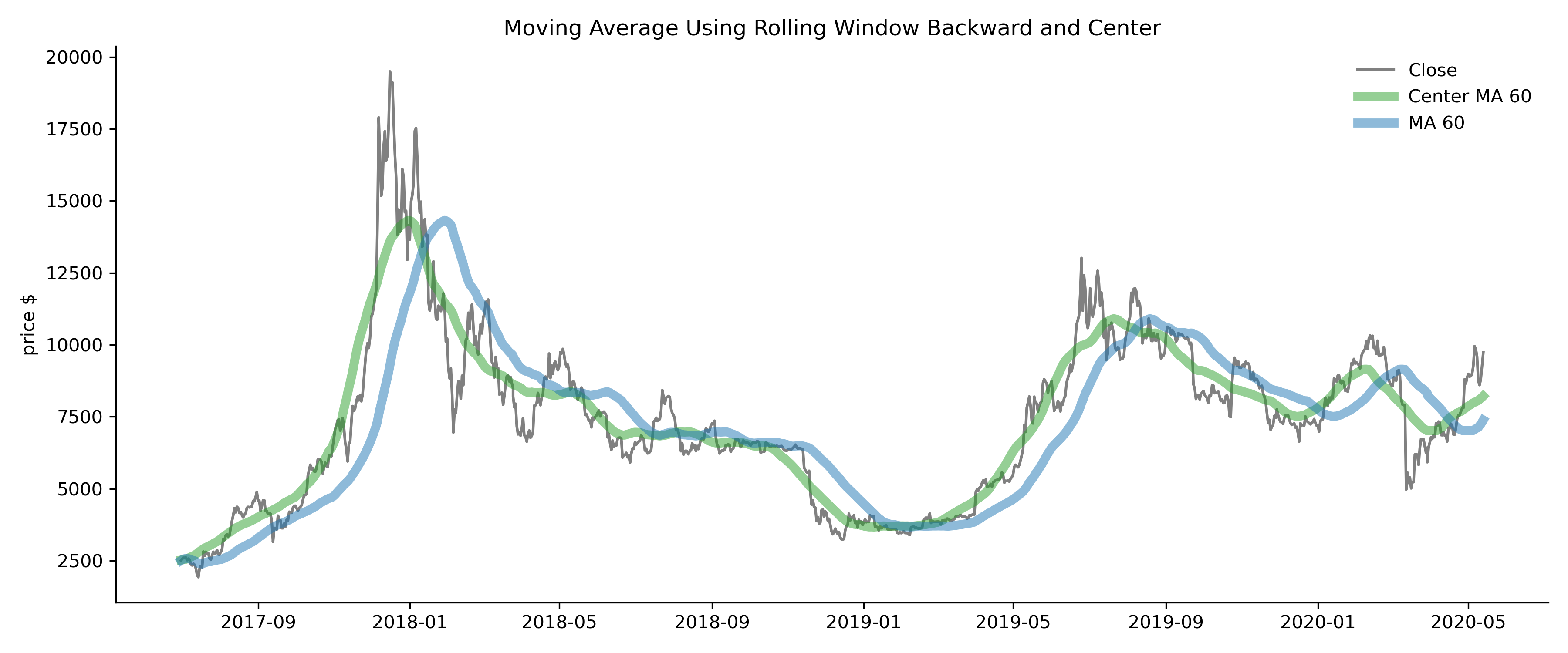
Moving average is usually calculated using backward window. This is intuitive because data usually are historical.
However, backward looking window calculated statistics has a lagging effect due to all but one of the data points are from the past.
If we want centered moving averages, we can specify by using the center parameter.
In the following example, we plot three lines: the grey line is the Bitcoin daily closing price, the green line is the 60-day centered moving average, and the blue line is the 60-day (backward) moving average. Notice that the centered moving average matches the Close price line without any shifting. Whereas the moving average line looks like it is shifted to the right, because it is using older data. You may wonder, how do we compute the backward moving averages for the oldest time points, and how do we compute the center moving averages for the newest time points? Although the default is min_periods=1 when there are fewer rows than the window size at the two ends, you can change that based on what makes sense in your problem.
import pandas_datareader.data as pdr
BTC = pdr.get_data_yahoo('BTC-USD', start=datetime(2010, 7, 16), end= datetime(2020, 10, 25)
Close = BTC.loc['2017-07-01':'2020-05-13','Close']
fig, ax = plt.subplots(1,1, figsize=(12,5))
ax.plot(Close,'grey',label= 'Close' )
ax.plot(Close.rolling(60).mean(),green,alpha=0.5,lw=5, label= 'Center MA 60')
ax.plot(Close.rolling(60,center=True).mean(),blue,alpha=0.5, lw=5,label= 'MA 60')
plt.ylabel('price $')
For SAS, for the moving average of a few data points, using lag function in the data step is sufficient. But for much longer time windows, we should use PROC EXPAND, or a SAS macro with base SAS.
We will skip the data preparation step. Note that although PROC SORT is not needed here because the data is already in chronological order, it is used as a reminder that the input to PROC EXPAND must be sorted. Note that the time column, date, must be listed in the ID statement.
The CONVERT statement specifies the names of the input and output variables. The TRANSMOUT= option specifies the method and parameters that are used to compute the rolling statistics. The METHOD=NONE option ensures that actual dataare used to compute the moving averages, rather than interpolated values, because the EXPAND procedure fits cubic spline curves to data by default.
PROC SORT DATA=btc; OUT=btc_sorted;
  BY date;
run;
PROC EXPAND DATA=btc_sorted OUT=out METHOD=NONE;
ID date;
CONVERT close = ma   / TRANSOUT=(MOVAVE 60);
CONVERT close = cma   / TRANSOUT=(CMOVAVE 60);
CONVERT close = wma  / TRANSOUT=(MOVAVE(1 2 3 4));
CONVERT close = ewma / TRANSOUT=(EWMA 0.3);
RUN;
PROC SGPLOT DATA=out CYCLEATTRS;
   SERIES X=date Y=ma   / NAME='MA'   LEGENDLABEL="MA(60)";
   SERIES X=date Y=cma   / NAME='CMA'   LEGENDLABEL="CMA(60)";
   SERIES X=date Y=wma  / NAME='WMA'  LEGENDLABEL="WMA(1,2,3,4)";
   SERIES X=date Y=ewma / NAME='EWMA' LEGENDLABEL="EWMA(0.3)";
   SCATTER X=date Y=y;
   keylegend 'MA' 'WMA' 'EWMA';
   XAXIS DISPLAY=(NOLABEL) GRID;
   YAXIS LABEL="CLOSING PRICE" GRID;
RUN;
Moving Averages and Trending Signals
Moving averages are often used for identifying trending signals. For example, real estate investors often use moving averages of real estate prices of metropolitan areas to learn the direction of the market. Moving averages are routinely used to remove seasonality in timeseries data with strong seasonal effect. To be able to apply different techniques in moving averages is essential in time series analysis and feature engineering.
Example below shows daily closing price, and moving averages in 20, 50, and 200 day rolling window. The wider the rolling window, the lines are smoother.
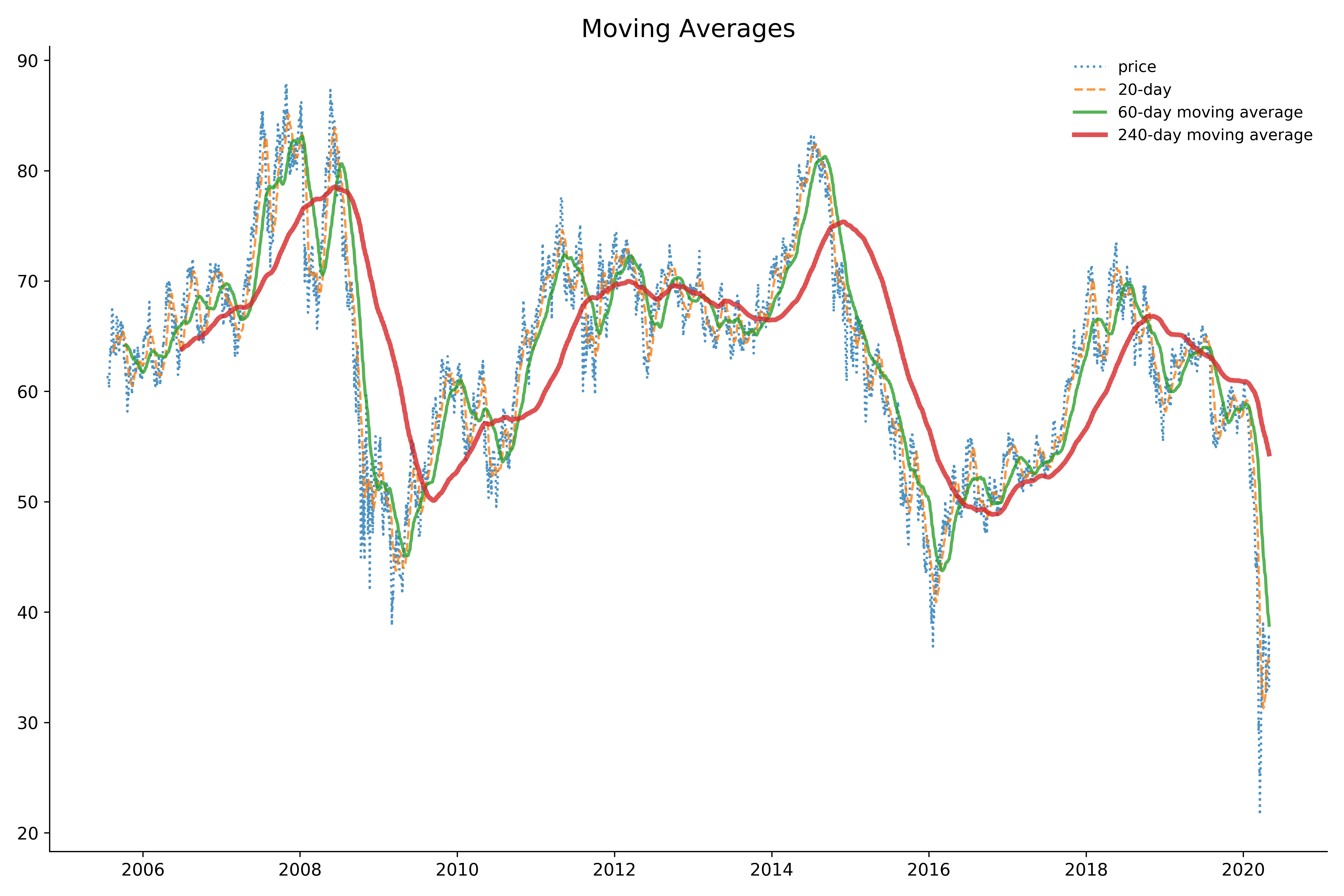
SP500_data = pdr.get_data_yahoo('^GSPC', start=start, end=date.today())
SP500 = SP500_data.loc['2005':]
ma20 = SP500.Close.rolling(20).mean()
ma50 = SP500.Close.rolling(50).mean()
ma200= SP500.Close.rolling(200).mean()
ma = pd.DataFrame({
    'price':SP500.Close,
    'ma20': ma20,
    'ma50': ma50,
    'ma200': ma200
})
# plotting
title = "Moving Averages"
fig, ax = plt.subplots(1,1, figsize=(12,8))
ax.plot(ma.price, label="price" ,alpha=0.8, linestyle=":")
ax.plot(ma['ma20'], label='20-day',alpha=0.8,linestyle="--")
ax.plot(ma['ma50'], label='50-day moving average',alpha=0.8,lw=2)
ax.plot(ma['ma200'], label='200-day moving average',alpha=0.8, lw=3)
ax.spines['top'].set_visible(False)
ax.spines['right'].set_visible(False)
plt.legend(frameon=False)
Moving Average Crossovers
Moving average crossovers are used widely in stock trade. Despite the efficient market hypothesis that markets are supposed to be rational and efficient, traders use moving averages and crossovers for trading strategies. Warren Buffet probably would not suggest any of these.
For technical analysis traders, when price or a shorter-term average crosses longer-term average, if it rises above then it is a buy signal, otherwise a sell signal.
On the other hand, another group of traders may argue that when price or a shorter-term average crosses longer-term average and rises above/below, the stock is overvalued/undervalued and should be sold/bought.
Below figure shows S&P 500 closing price and 20-day moving average in the first five months and eight days of 2020, when the Covid-19 pandemic spread across the world.
Although the price did not hit the lowest until March 23, various technical analysis indicators might have compelled some to begin selling weeks before.
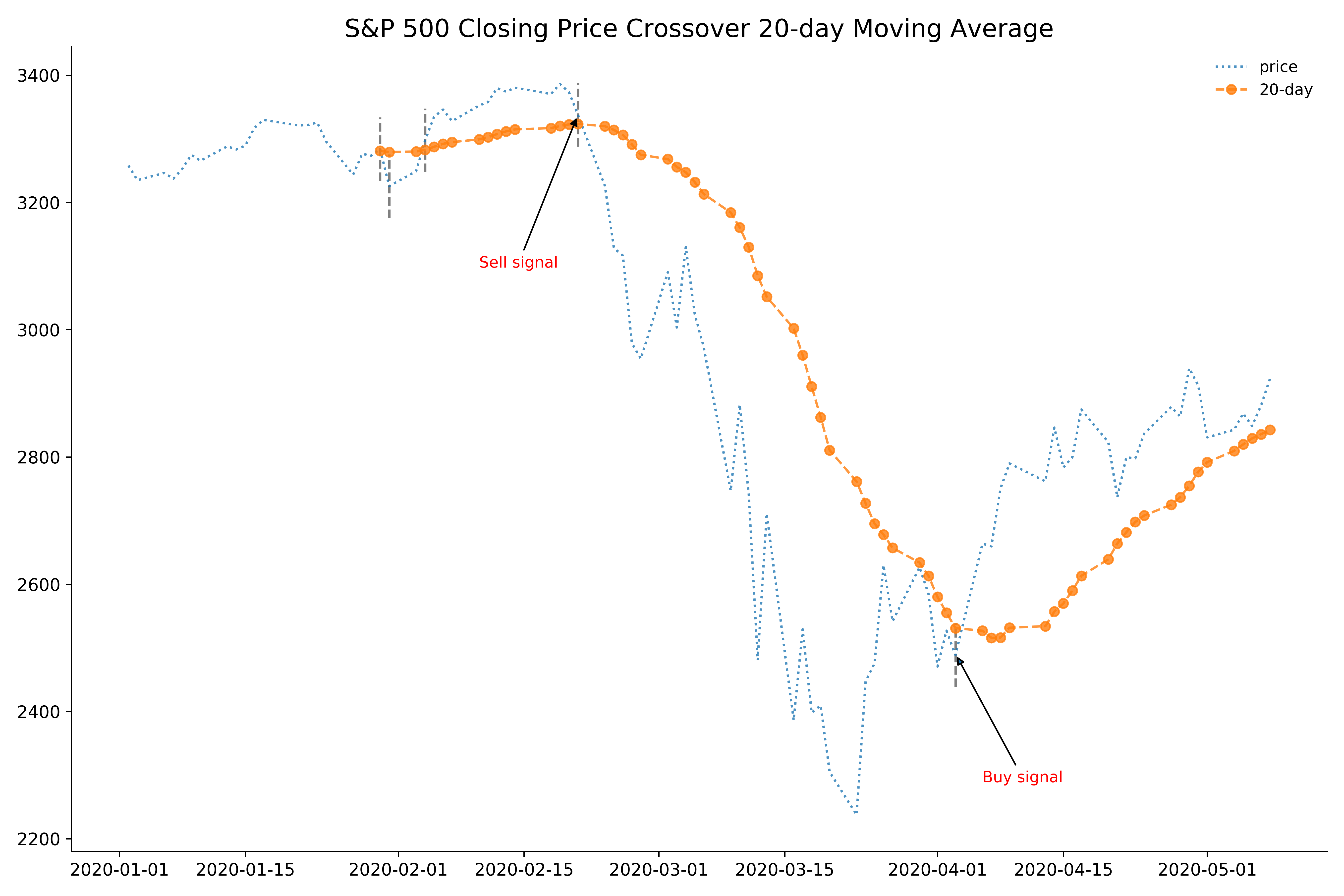
from datetime import timedelta
SP500 = SP500_data.loc['2020':]
ma20 = SP500.Close.rolling(20, center = False).mean()
ma = pd.DataFrame({
    'price':SP500.Close,
    'ma20': ma20})
# compute crossover dates
larger = ma20 < ma.price
larger_previous = larger.shift(1)
crossing = np.where(abs(larger-larger_previous)==1)
ma_crossing = ma.iloc[crossing].copy()
print(ma_crossing)
Out:
              price     ma20
Date
2020-01-30 3283.660 3280.837
2020-01-31 3225.520 3279.220
2020-02-04 3297.590 3282.489
2020-02-24 3225.890 3319.692
2020-04-06 2663.680 2526.790
# to prevent 3-day gap, use Friday data instead of Monday
for i in range(ma_crossing.shape[0]):
    if ma_crossing.index[i].weekday()==0:
        ma_crossing.loc[ma_crossing.index[i],'date']= ma_crossing.index[i]-timedelta(days=3)
        ma_crossing.loc[ma_crossing.index[i],'price']= ma.price.loc[ma_crossing.index[i]-timedelta(days=3)]
    else:
        ma_crossing.loc[ma_crossing.index[i],'date']= ma_crossing.index[i]
        ma_crossing.loc[ma_crossing.index[i],'price'] = ma_crossing.loc[ma_crossing.index[i],'price']

title = "S&P 500 Closing Price Crossover 20-day Moving Average"
fig, ax = plt.subplots(1,1, figsize=(12,8))
ax.plot(ma.price, label="price" ,alpha=0.8, linestyle=":")
ax.plot(ma['ma20'], label='20-day',alpha=0.8,linestyle="--",marker="o")
ax.vlines(ma_crossing.date,ma_crossing.price-150, ma_crossing.price+150,linestyle='--')
title = "S&P 500 Closing Price Crossover 20-day Moving Average"
fig, ax = plt.subplots(1,1, figsize=(12,8))
ax.plot(ma.price, label="price" ,alpha=0.8, linestyle=":")
ax.plot(ma['ma20'], label='20-day',alpha=0.8,linestyle="--",marker="o")
ax.vlines(ma_crossing.date,ma_crossing.price-50, ma_crossing.price+50,linestyle='--',color="0.5")
ax.annotate("Sell signal", xy=(ma_crossing.date[-2],ma_crossing.price[-2]), xycoords='data', xytext=(datetime(2020,2,10),ma_crossing.price[-3]-200), textcoords='data',color='r', arrowprops=dict(fc='k', arrowstyle="-|>"))
ax.annotate("Buy signal", xy=(ma_crossing.date[-1],ma_crossing.price[-1]+2), xycoords='data',
                  xytext=(datetime(2020,4,6),ma_crossing.price[-1]-200), textcoords='data',color='r',arrowprops=dict(arrowstyle="-|>"))
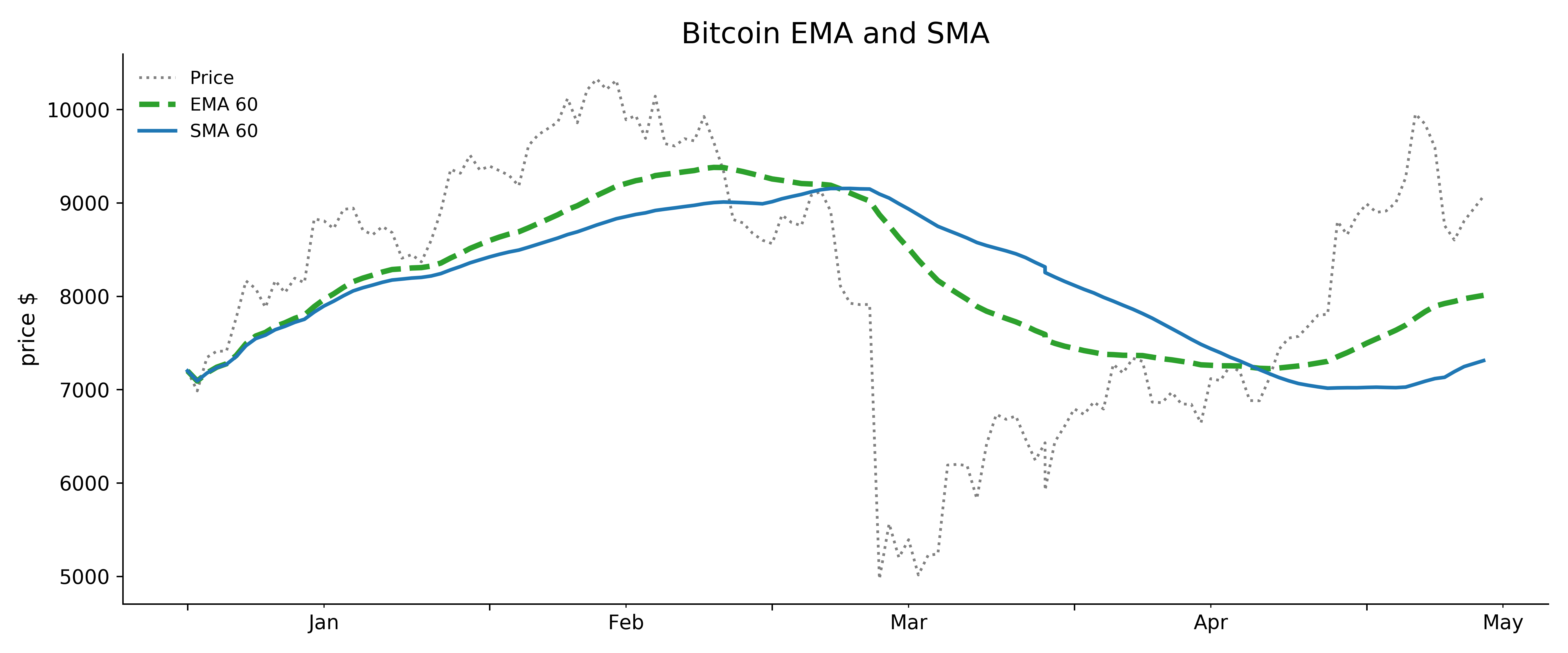
Exponentially Smoothing
Exponentially smoothing, also called “exponential weighted average”, is a commonly used smoothing method. It is like moving average in that both are window functions. The only difference is that exponential smoothing assign exponentially decreasing weights over time, where the weight is 1- α. The formula is:

The relationship between window size and α is α=2/(window size+1). There are many smoothing methods. The simplest is exponentially weighted moving average (EWMA). We demonstrate the use of simple moving average and EWMA in two examples.
import matplotlib.ticker as ticker
import matplotlib.dates as mdates
from matplotlib.ticker import NullFormatter
from matplotlib.dates import MonthLocator, DateFormatter
Close = BTC.loc['2020':'2020-05-13','Close']
ma60 = Close.rolling(60, min_periods=1).mean()
EMA =  Close.ewm(span=60).mean()
title = 'Bitcoin EMA and SMA'
fig, ax = plt.subplots(1,1, figsize=(12,5))
ax.plot(Close,'grey',linestyle=':',label= 'Price')
ax.plot(EMA,green,lw=3,linestyle="--", label= 'EMA 60')
ax.plot(ma60,blue, lw=2,label= 'SMA 60')
ax.xaxis.set_major_locator(MonthLocator())
ax.xaxis.set_minor_locator(MonthLocator(bymonthday=15))
ax.xaxis.set_major_formatter(NullFormatter())
ax.xaxis.set_minor_formatter(DateFormatter('%b'))
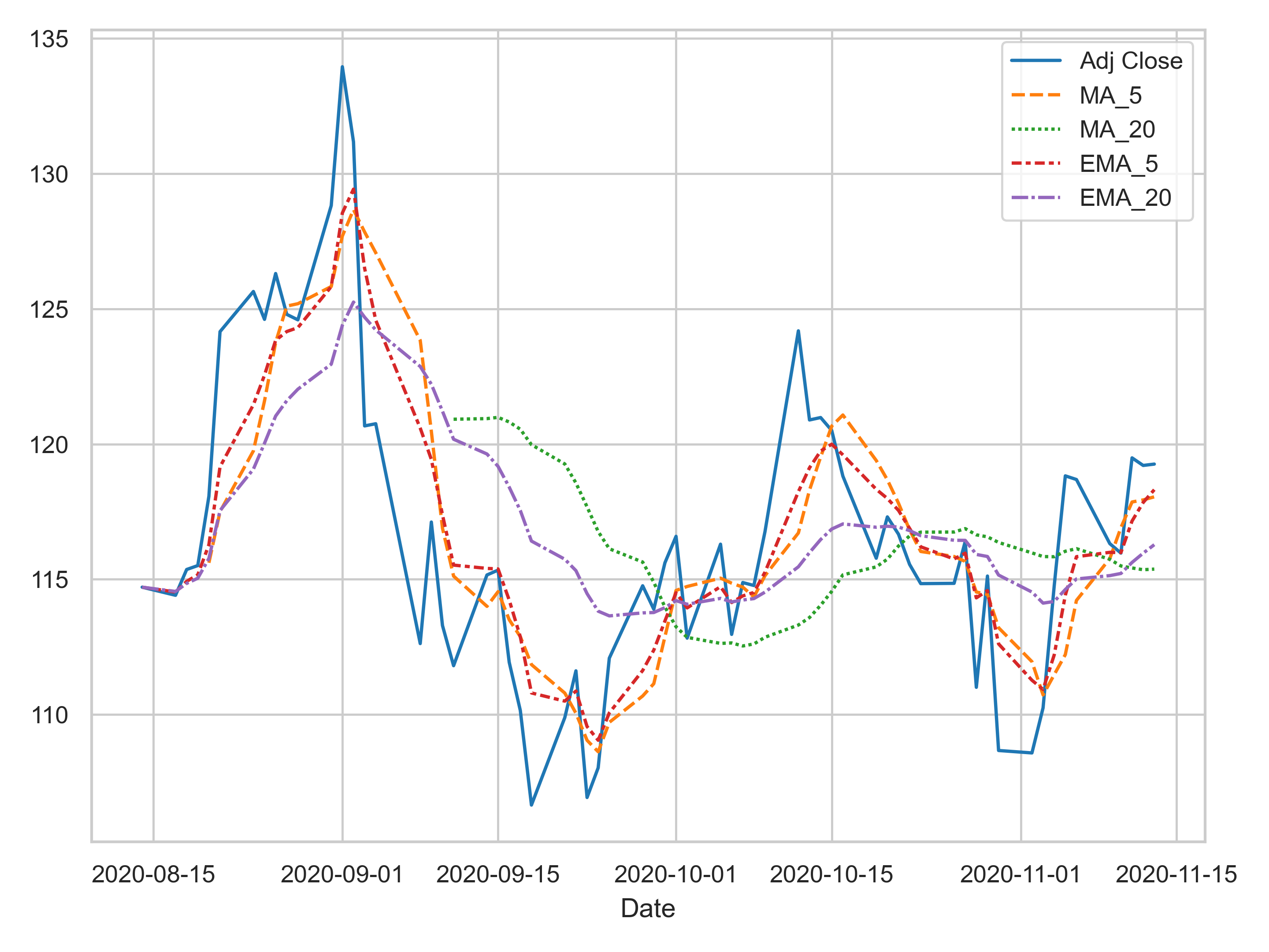
import pandas_datareader.data as pdr
AAPL = pdr.get_data_yahoo('AAPL', start=pd.Timestamp(2020, 8,14), end=pd.Timestamp(2020, 11,14))
def processEMA(ts_data):
    ts_data.sort_values('Date', inplace=True)
    # compute moving averages
    ma_list = [5, 20]
    for ma in ma_list:
        ts_data['MA_' + str(ma)] = ts_data['Adj Close'].rolling(ma).mean()
    # compute exponential moving averages
    for ma in ma_list:
        ts_data['EMA_' + str(ma)] = ts_data['Adj Close'].ewm(span=ma).mean()
processEMA(AAPL)
sns.set_style("whitegrid")
sns.set_context("paper")
sns.lineplot(data= AAPL.iloc[:,5:])
Notice that the exponentially smoothed (dash-dot lines) are more responsive to daily price than simple moving average (dash lines) because of greater weights on more recent data points.
In SAS, using PROC EXPAND is very simple to create exponential moving average. But we need to provide the weight muliplier instead of window width.
Weighted multiplier =2÷(selected time period+1)
For the 5 days EWMA, weight =2÷(5+1) =0.33
For the 20 days EWMA, weight =2÷(20+1) =0.095
PROC EXPAND DATA=APPL OUT=out METHOD=NONE;
ID date;
CONVERT close = MA5   / TRANSOUT=(MOVAVE 5);
CONVERT close = MA20   / TRANSOUT=(MOVAVE 20);
CONVERT close = EWMA5 / TRANSOUT=(EWMA 0.3);
CONVERT close = EWMA20 / TRANSOUT=(EWMA 0.095);
RUN;
PROC SGPLOT DATA=out CYCLEATTRS;
   SERIES X=date Y=MA5   / NAME='MA5'   LEGENDLABEL="MA(5)";
   SERIES X=date Y=MA20   / NAME='MA20'   LEGENDLABEL="MA(20)";
   SERIES X=date Y=EWMA5 / NAME='EWMA5' LEGENDLABEL="EWMA(0.3)";
   SERIES X=date Y=EWMA20 / NAME='EWMA20' LEGENDLABEL="EWMA(0.095)";
   SCATTER X=date Y=y;
   keylegend 'MA5' 'MA20' 'EWMA5' 'EWMA20';
   XAXIS DISPLAY=(NOLABEL) GRID;
   YAXIS LABEL="CLOSING PRICE" GRID;
RUN;
A Note for SAS Users
SAS users can choose PROC EXPAND, PROC TIMEDATA or PROC TIMESERIES, and even PROC MEANS to manipulate data to any frequency.
When the window width is an odd number, then there is no difference between SAS PROC EXPAND CMOVAVE and Python pandas center moving averages. But when the width is an even number, then they are different. One more lead value than lag value is included in the time window in PROC EXPAND CMOVAVE.
For example, the result of the CMOVAVE 4 operator is:
SAS: y_t=(x_(t-1)+x_t+x_(t+1)+ x_(t+2))/4
Whereas pandas rolling(4, center = True) takes one more lag than lead.
Python: y_t=(x_(t-2)+x_(t-1)+x_t+ x_(t+1))/4