This post consists of a few timeseries examples from my upcoming book on statistical and machine learning using Python, sequal to my co-authored book Python for SAS User
Expanding windows
Expanding window statistics are useful for cumulative statistics like month-to-date moving sum, YTD moving average, etc. For each row, it computes statistics with all the data available up to that point in time. It is called “expanding window” probably because we are using increasing larger window as we go down the rows. These can be useful when we want to use all historical data instead of a certain number of them, for example, customer total spend and credit card total points since account opening, user cumulative rating on a sharing economy app, etc.
Similar to SAS cumulative statistics, pandas .expanding() object returns value of the statistic with all the data available up to that point in time. Like rolling, expanding window is not limited to time series. It applies to all pandas DataFrame or Series objects. Expanding is implemented in pandas as a special case of rolling statistics.
In the following example, we show that expanding returns statistics that are the same as cumsum() when min_periods =1. The difference is that expanding window statistics ignores NaN values whereas cumsum() returns NaN when encounter one. So if you have missing values in the data, you may want to use expanding instead of cumsum.
 idx=pd.date_range('1/1/2020', periods=5)
 s = pd.Series([2,3, np.nan, 10,20], index=idx)
 s
[Out]:
2020-01-01     2.0
2020-01-02     3.0
2020-01-03     NaN
2020-01-04    10.0
2020-01-05    20.0
Freq: D, dtype: float64

 s.expanding(min_periods=1).sum()
[Out]:

2020-01-01     2.0
2020-01-02     5.0
2020-01-03     5.0
2020-01-04    15.0
2020-01-05    35.0
Freq: D, dtype: float64

 s.cumsum()
2020-01-01     2.0
2020-01-02     5.0
2020-01-03     NaN
2020-01-04    15.0
2020-01-05    35.0
Freq: D, dtype: float64
It may be of interest sometimes to keep tract of the total number of non-null values at each record. For example, a company may want to know the cumulative number of payments or records any account may have. Listing 1- 33, using the same example data as above, shows such an example.
 idx = pd.to_datetime(['2021-01-01', '2021-01-03', '2021-01-05', '2021-01-06','2021-01-08'])
 df.index = idx
 df
[Out]:
 s.expanding(min_periods=1 ).count()
[Out]:
2020-01-01    1.0
2020-01-02    2.0
2020-01-03    2.0
2020-01-04    3.0
2020-01-05    4.0
Freq: D, dtype: float64
Conceptually, rolling statistics should be the same as expanding ones when the window width is set to be the length of the timeseries, because both include all historical data.
For examples:
 s.rolling(window=len(s), min_periods=1).mean()
 s.expanding(min_periods=1).mean()
And the following two calls are also equivalent:
 s.rolling(window=len(s), min_periods=1,center=True).mean()
 s.expanding(min_periods=1, center=True).mean()
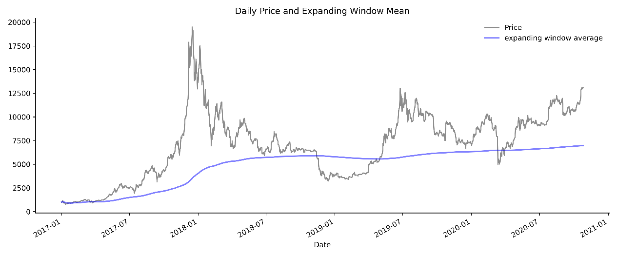
As one can expect, when window width is less than time series data, expanding moving average is much more stable and much less sensitive to current data than rolling window average. In Figure 1- 5, using the same Bitcoin data, we plot the expanding window average from year 2017 overlay with daily closing price.