This post consists of a few timeseries regression examples from my upcoming book on statistical and machine learning using Python, also to be published by Apress,as my co-authored book Python for SAS User. There are two main categories of models for time series data:
- Various variations of OLS type of regression y = a + b*x. To account for residual serial correlation, Newey-West standard errors may be used.
- Time series model, such as ARIMAX, SARIMAX
We will begin with some data analysis and then get into modeling.
Data Visualization
When we look at the timeseries data in various types of plots, we should take note of the following:
- Is mean-reverting or has explosive behavior
- Does it have a time trend
- Seasonality
- Structrural breaks
Test for Structural Breaks
It could be argued that the most important assumption of any time series model is that the underlying process is the same across all observations in the sample. Because of this, we should analyze carefully time series data with abrupt changes visually. Researching the history of the data and its context should go hand in hand with statistical analysis.
The Chow test is commonly used to test for structural change in some or all of the parameters of a model in cases where the disturbance term is assumed to be the same in both periods.
The Chow Test tests if the weights in two different regression models are the same. In other words, it tests if the model before the possible break point is the same as the model after the possible break point. The alternative hypothesis is the model fitting each periods are different.
It formally tests this by performing an F-test on the Chow Statistic which is (RSS_pooled - (RSS1 + RSS2))/(number of independent variables plus 1 for the constant) divided by (RSS1 + RSS2)/(Number of observations in subsample 1 + Number of observations in subsample 2 - 2*(number of independent variables plus 1 for the constant).
The models in each of the models (pooled, 1, 2) must have normally distributed error with mean 0, as well as independent and identically distributed errors, to satisfy the Gauss-Markov assumptions.
One of the problems of Chow’s test is that our model may detect too many breaks. In situations like this, we have to go back to the history of the data and its context, and apply judgement in combination with test results. To use Chow’s test most effecitvely, we probably should have an idea the ballpark where we want to test.
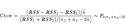
Data: Food and energy CPI
Looking at economic activity data year over year (or sometimes quarter over quarter) is a routine exercise for analysts who work with macroeconomic data, and business performance data. Tranformating the target variable using YoY often makes the time series stationary and non-serial correlated. Stationary target variable makes modeling easier because it is reduces chances of spurious regression and it is easier to isolate problems. Why? Let’s make an analogy, when you have two objects, it is easier to see what is happening if you keep one object relatively fixed (stationary) instead of both are moving.
Food and energy (along with housing) are the most important factors in daily life. We use CPI data from FRED for our first example, using .to_frame().join([meat,energy]) to combine the three time series together: urban meat prices, all food prices, and energy prices.
To avoid seeing too much volatility, we first convert the monthly data to quarterly by using .resample(‘Q’).mean(), then chain it with .pct_change(4). This gives us a quick way to compare a few time series in year over year change.
pd.options.display.float_format = '{:10,.1f}'.format
fred = fred(api_key='your key')
from fredapi import Fred as fred
import matplotlib.pyplot as plt
import seaborn as sns
sns.set()
meat=fred.get_series('CWSR0000SAF112')
meat.name ='meat'
food=fred.get_series('CPIUFDNS')
food.name = 'food'
energy=fred.get_series('CUSR0000SEHF')
energy.name = 'energy'
title = "energy,meat and all food CPI"
df = food.to_frame().join([meat,energy]).resample('Q').mean().pct_change(4)
df.plot(figsize=(15,5), alpha=0.8, linewidth=3)
plt.title(title)
# plt.savefig(r".\TimeSeries\images\food_cpi.png")
plt.show()
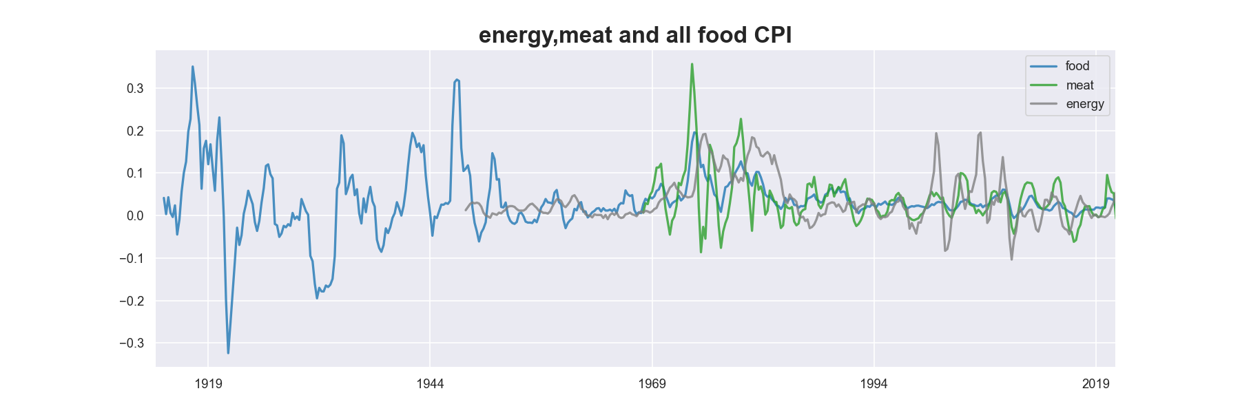
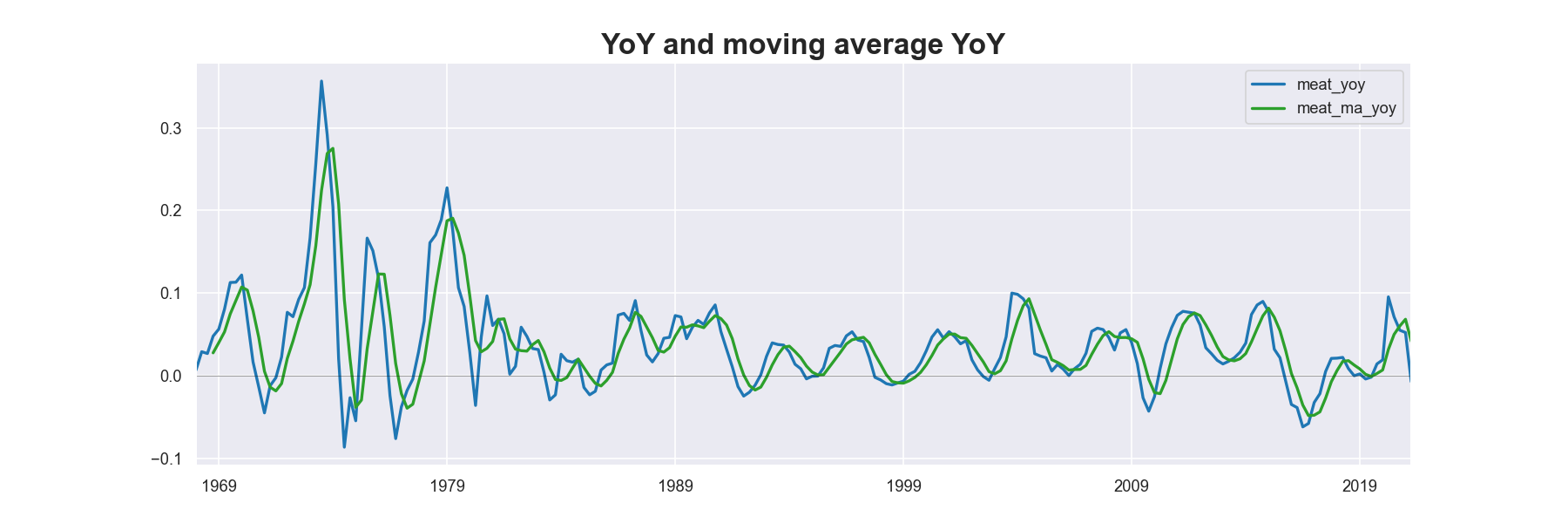
Data Transform
A variation of YoY transformation is moving average YoY, which first takes moving average before computing year over year. Only one line of code is need to accomplish this. Again, .resample(‘Q’).mean() changes frequency of the data from monthly to quarterly. .rolling(4).mean() takes four-quarter moving average, followed by .pct_change(4) to make it year over year change.
title = "CPI moving average YoY"
food.to_frame().join([meat,energy]).resample('Q').mean().rolling(4).mean().pct_change(4).plot(figsize=(15,5),linewidth=2, color=[blue, green,'grey'])
plt.title(title,fontdict={'fontsize': 20, 'fontweight': 'bold'})
If we have many series and cannot plots them in one chart, we may want to use the following code. To make the plots more informative, we can annotate them with statistics such as historical mean. </span> takes four-quarter moving average, followed by .pct_change(4) to make it year over year change.
fred_series = ['CWSR0000SAF112','CPIUFDNS','CUSR0000SEHF' ]
series_names = ['meat','food','energy']
series_dict = dict(zip(fred_series,series_names))
# get series together and save them in a dataframe
s_list =[]
for i in fred_series:
s = fred.get_series(i)
s_list.append(s)
s_df = pd.concat(s_list, axis=1) #convert a list of series to dataframe
s_df.columns=series_names
# transform the entire dataframe
s_yoy =s_df.resample('Q').mean().pct_change(4)
MEAN = s_yoy.mean()
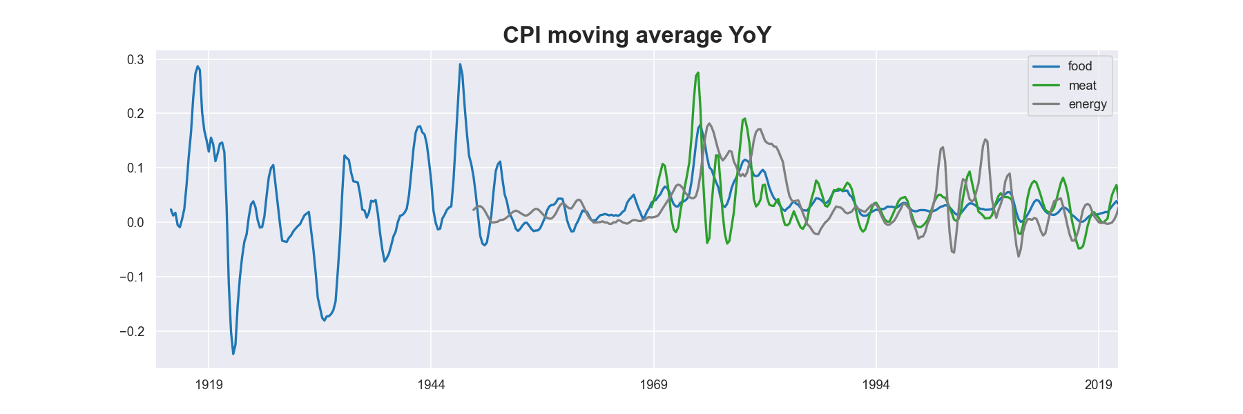
for i in fred_series:
NAME = series_dict[i]
title = "CPI " + NAME + ' '+ i
fig, ax = plt.subplots(1,1)
s_yoy[NAME].dropna(axis=0).plot(label=NAME,color=blue, ax=ax)
left_pos = s_yoy[NAME].first_valid_index()
right_pos = s_yoy[NAME].last_valid_index()
plt.hlines(MEAN[NAME], xmin=left_pos,xmax=right_pos, linestyles=":", alpha=0.3)
# annotate with historical mean
ax.text(s_yoy[NAME].first_valid_index(),MEAN[NAME], '$mean: {:.1f}$%'.format(100*MEAN[NAME]))
plt.hlines(0, xmin=left_pos,xmax=right_pos, lw=4, alpha=0.5, color='white')
plt.legend(frameon=False)
plt.title(title)
plt.show()
Note 1. 1900 - 1914 The Gold standard and stability 2. 1915 - 1924 Inflation - World War I 3. 1925 - 1939 Deflation - Interwar instability 4. 1949 - 1970 Moderate inflation - Bretton Woods and the Dollar standard 5. 1971 - 1979 Highly variable inflation - Floating exchange rates, OPEC 6. 1980 - 2000 *Disinflation* - Greater central bank independence
deflation is a decrease in general price levels throughout an economy. Deflation, which is the opposite of inflation, is mainly caused by shifts in supply and demand. disinflation is what happens when price inflation slows down temporarily. Disinflation shows the rate of change of inflation over time.
Because time series transformation is often used in feature engineering in models, we may need to merge the transformed data with the level data.
Note When merging data back, it is important to check by looking at the data, and reading the numbers. Python is easy to use, and is also very easy to make mistake with. For example, when using .join, default method is on index, if the series have different frequency, then nothing will be merged.
df = food.to_frame().join([meat,energy]).resample('Q').mean()
yoy_df = df.pct_change(4)
ma_yoy_df = df.rolling(4).mean().pct_change(4)
df = df.join(yoy_df, rsuffix='_yoy')
df = df.join(ma_yoy_df, rsuffix='_ma_yoy')
title = "YoY and moving average YoY"
df[['meat_yoy','meat_ma_yoy']].dropna(how='all',axis=0).plot(figsize=(15,5),linewidth=2, color=[blue, green])
plt.title(title,fontdict={'fontsize': 20, 'fontweight': 'bold'})
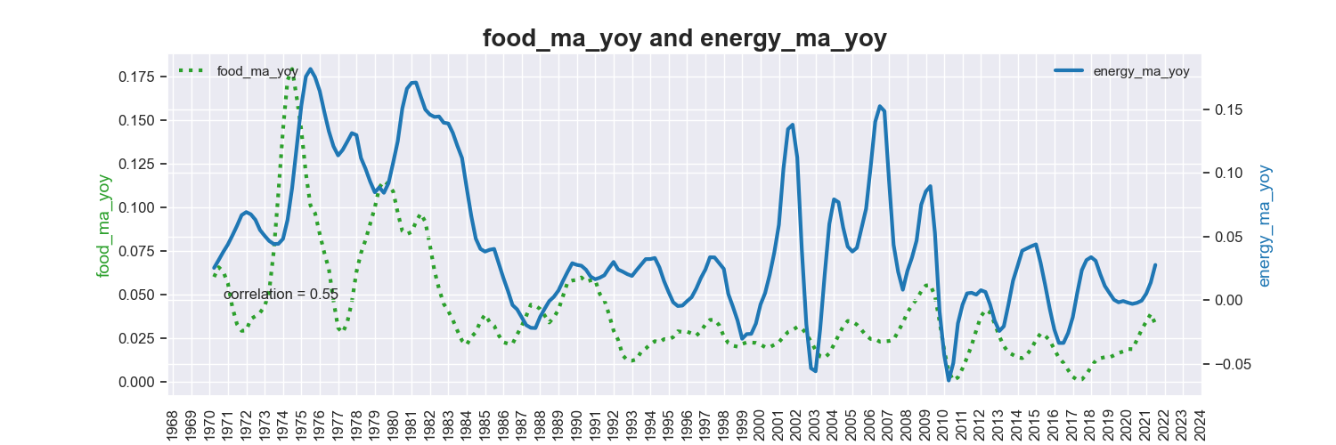
Bi-variate Plots Check for Economic Intuition
def plot_2_ts(data, x, y, year):
    '''
    plot 2 time series using secondary axis
    y is plotted with solid blue line
    x is in dotted green line
    annotated with correlation
    year is the beginning year
    '''
    temp = data.loc[str(year):, [x]+[y]].dropna(how='any', axis=0).copy()
    corr = np.round(temp.corr().iloc[0,1],2)
    print("corr \n",corr)
    title = x + " and " + y
    fig, ax1 = plt.subplots(1,1,figsize=(15,5))
    ax2 = ax1.twinx()
    ax1.plot(temp.index, temp[x], color=green, label=x,linestyle=":", lw=3)
    ax2.plot(temp.index, temp[y], color=blue, label=y, lw=3)
    ax1.set_ylabel(x, color=green)
    ax2.set_ylabel(y, color=blue)
    ax2.xaxis.set_major_locator(YearLocator()) #frequency
    ax2.xaxis.set_major_formatter(DateFormatter('%Y'))
    ax2.text(temp.index[2],temp[y].min(), "correlation = %s"%str(corr))
    ax1.tick_params(axis='x', labelrotation = 90)
    ax2.tick_params(axis='x', labelrotation = 90)
    ax1.legend(frameon=False, loc=2)
    ax2.legend(frameon=False, loc=1)
    plt.xticks(fontsize=5)
    plt.title(title,fontsize=20, fontweight ='bold')
plot_2_ts(df, x= "food_ma_yoy", y = "energy_ma_yoy", year=1970)
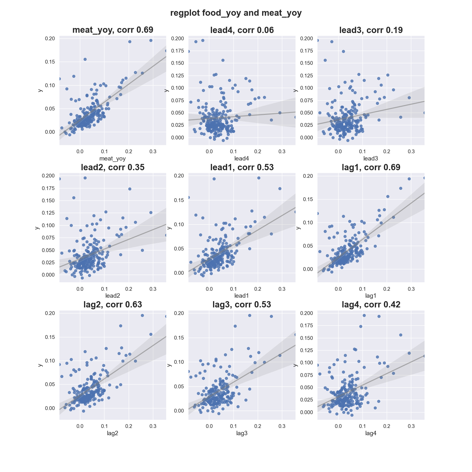
Regression Analysis
After preparing the data, we may want to do some simple regression analysis for feature selection. Below is an example that looks at various lags and leads to find which is the most correlated one with the target.
def regplots(x, y, data):
    df = data[[y,x]].dropna(how='all', axis=0).copy()
    df.rename({y:'y'}, inplace=True, axis=1)
    df['lead1'] = df[x].shift(-1)
    df['lead2'] = df[x].shift(-2)
    df['lead3'] = df[x].shift(-3)
    df['lead4'] = df[x].shift(-4)
    df['lag1'] = df[x].shift(1)
    df['lag2'] = df[x].shift(2)
    df['lag3'] = df[x].shift(3)
    df['lag4'] = df[x].shift(4)
    corrs = np.round(df.corr()['y'][1:],2)
    print("correlation is:/n", corrs)
    cols = [x,'lead4','lead3','lead2','lead1','lag1','lag2','lag3','lag4']
    lwargs = {'color':'grey', 'alpha':0.6}
    lwargs2 = {'color':'k', 'alpha':0.6}
    fig, ax = plt.subplots(3,3, figsize=(15,15))
    sns.regplot(x=df[cols[0]], y=df.y, data=df, ax=ax[0,0],line_kws=lwargs).set_title("%s, corr %s"%(cols[0],str(corrs[cols[0]])))
    sns.regplot(x=df[cols[1]], y=df.y, data=df, ax=ax[0,1],line_kws=lwargs).set_title("%s, corr %s"%(cols[1],str(corrs[cols[1]])))
    sns.regplot(x=df[cols[2]], y=df.y, data=df, ax=ax[0,2],line_kws=lwargs).set_title("%s, corr %s"%(cols[2],str(corrs[cols[2]])))
    sns.regplot(x=df[cols[3]], y=df.y, data=df, ax=ax[1,0],line_kws=lwargs).set_title("%s, corr %s"%(cols[3],str(corrs[cols[3]])))
    sns.regplot(x=df[cols[4]], y=df.y, data=df, ax=ax[1,1],line_kws=lwargs).set_title("%s, corr %s"%(cols[4],str(corrs[cols[4]])))
    sns.regplot(x=df[cols[5]], y=df.y, data=df, ax=ax[1,2],line_kws=lwargs).set_title("%s, corr %s"%(cols[5],str(corrs[cols[5]])))
    sns.regplot(x=df[cols[6]], y=df.y, data=df, ax=ax[2,0],line_kws=lwargs).set_title("%s, corr %s"%(cols[6],str(corrs[cols[6]])))
    sns.regplot(x=df[cols[7]], y=df.y, data=df, ax=ax[2,1],line_kws=lwargs).set_title("%s, corr %s"%(cols[7],str(corrs[cols[7]])))
    sns.regplot(x=df[cols[8]], y=df.y, data=df, ax=ax[2,2],line_kws=lwargs).set_title("%s, corr %s"%(cols[8],str(corrs[cols[8]])))
    title ="regplot %s and %s"%(y,x)
    plt.suptitle(title,fontsize=20, fontweight ='bold')
    plt.subplots_adjust(top=0.925, hspace=0.25)
    plt.savefig(r".\Volume2\TimeSeries\images\%s.png"%title)
regplots(x='meat_yoy',y='food_yoy',data=df)
Out:
correlation is:
meat_yoy   0.690
lead1      0.530
lead2      0.350
lead3      0.190
lead4      0.060
lag1       0.690
lag2       0.630
lag3       0.530
lag4       0.420
From the correlation and regression analysis, we see that without lead or lag the correlation between food and meat is the highest.
Below plots show that food price change is more often a leading indicator for energy price change. However,
- When the target variable leads a input variable, the predicted will lag behind the actual.
- When target leads a input, we cannot no longer call the input as a “driver”, as it implies causality.
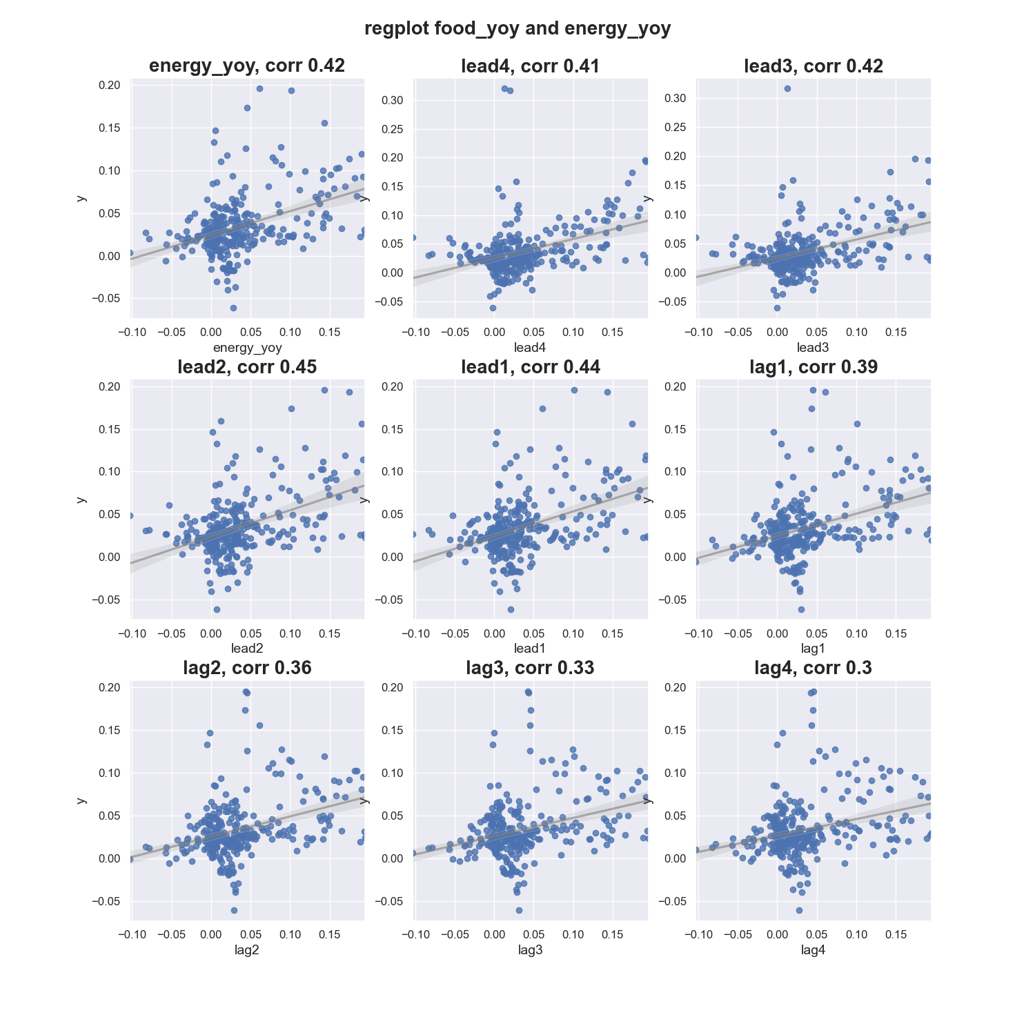
OLS Regression
We run a simple OLS regression using meat_yoy and energy_yoy to predict food_yoy.
import statsmodels.api as sm
from statsmodels.stats.stattools import durbin_watson
x1 = 'meat_yoy'
x2 = 'energy_yoy'
y =  'food_yoy'
ts = df[[x1,x2,y]].copy()
ts.dropna(how='any', axis =0, inplace=True)
X = ts[[x1,x2]].copy()
X = sm.add_constant(X)
model = sm.OLS(ts[y],ts[[x1,x2]]).fit()
model.summary()
[Out]:
                            OLS Regression Results
==============================================================================
Dep. Variable:               food_yoy   R-squared:                       0.628
Model:                            OLS   Adj. R-squared:                  0.625
Method:                 Least Squares   F-statistic:                     178.5
Date:                Sun, 16 May 2021   Prob (F-statistic):           4.28e-46
Time:                        17:44:34   Log-Likelihood:                 536.07
No. Observations:                 214   AIC:                            -1066.
Df Residuals:                     211   BIC:                            -1056.
Df Model:                           2
Covariance Type:            nonrobust
==============================================================================
                 coef    std err          t      P>|t|      [0.025      0.975]
------------------------------------------------------------------------------
const          0.0168      0.002      9.058      0.000       0.013       0.020
meat_yoy       0.3547      0.024     15.009      0.000       0.308       0.401
energy_yoy     0.2186      0.023      9.472      0.000       0.173       0.264
==============================================================================
Omnibus:                       82.989   Durbin-Watson:                   0.222
Prob(Omnibus):                  0.000   Jarque-Bera (JB):              390.244
Skew:                           1.458   Prob(JB):                     1.82e-85
Kurtosis:                       8.939   Cond. No.                         18.3
==============================================================================
Model Evalulation 1: Residual Autocorrelation and Stationarity
From the regression results, we see that DW is 0.222. Ideally DW should be close to 2. A rule of thumb is that test statistic values in the range of 1.5 to 2.5 are relatively normal. Close to 0 DW means the residual is positively auto-correlated. Close to 4 implies negative autocorrelation.
Autoregressive relationships are very common in time series. For example, when prices are increasing, it is likely to increase for a few years. This is what some may call “momemtum”.
In context such as stock trading, strong autocorrelation shows if there is a momentum factor associated with a stock and a suitable trading strategy may be used to explore the autocorrelation.
Autocorrelation does not impact coefficient values from OLS. It impacts the estimate of the errors in significance testing. Because one of the assumptions for OLS parameter testing is independence of errors, violating this assumption makes the the standard errors smaller than they actuarlly are.
Similarly, non-stationary residual can make us underestimate standard errors of the coefficent estimates. We use augmented Dicky-Fuller test to test resdual stationarity.
from statsmodels.tsa.stattools import adfuller
stationary_test_result = adfuller(model.resid)
print('ADF Statistic: %f' % stationary_test_result[0])
print('p-value: %f' % stationary_test_result[1])
[Out]:
ADF Statistic: -2.178328
p-value: 0.214205
There are mainly three methods to correct these problems.
One of the methods to correct the problem is to use heteroskedasticity and autocorrelation consistent (HAC) standard errors such as Newey-West ( Newey, Whitney K., and Kenneth D. West. “A Simple, Positive Semi-definite, Heteroskedasticity and Autocorrelation Consistent Covariance Matrix”. Econometrica 55.3 (1987): 703–708.) standard errors. By adding cov_type=’HAC’ to the fit method.
In the code below, to add the intercept term, sm.tools.add_constant(X) is used, which is equivalent to X = sm.add_constant(X) The new model summary shows that the standard errors now are larger. For example, for meat_yoy the std err went from 0.024 to 0.054. As a result, the coefficient estimate confidence intervals are wider.
X = ts[[x1,x2]].copy()
sm.OLS(ts[y], sm.tools.add_constant(X)).fit(cov_type='HAC',cov_kwds={'maxlags':2})
model.summary()
[Out]:

                            OLS Regression Results
==============================================================================
Dep. Variable:               food_yoy   R-squared:                       0.628
Model:                            OLS   Adj. R-squared:                  0.625
Method:                 Least Squares   F-statistic:                     43.12
Date:                Sun, 16 May 2021   Prob (F-statistic):           1.98e-16
Time:                        19:24:59   Log-Likelihood:                 536.07
No. Observations:                 214   AIC:                            -1066.
Df Residuals:                     211   BIC:                            -1056.
Df Model:                           2
Covariance Type:                  HAC
==============================================================================
                 coef    std err          z      P>|z|      [0.025      0.975]
------------------------------------------------------------------------------
const          0.0168      0.002      8.954      0.000       0.013       0.021
meat_yoy       0.3547      0.054      6.629      0.000       0.250       0.460
energy_yoy     0.2186      0.058      3.751      0.000       0.104       0.333
==============================================================================
Omnibus:                       82.989   Durbin-Watson:                   0.222
Prob(Omnibus):                  0.000   Jarque-Bera (JB):              390.244
Skew:                           1.458   Prob(JB):                     1.82e-85
Kurtosis:                       8.939   Cond. No.                         18.3
==============================================================================
Our goal is here is to get the right standard error for the coefficients. Since the p-values are extremely small even under the Newy-West errors in the presence of serial correlation and/or heteroskedasticity, we can conclude the model estimates are not significantly influenced by serial correlation and therefore appropriate for use. However, there is always a possibility that the model is not the right one for this data.
Newey-West standard errors is the simplest serial correlation corrections to implement for a simple OLS because it does not change the model if the parameters are significant. Depending on model purpose, OLS may be the preferred model, or sometimes we may prefer using a time series ARMA model to correct for autocorrelation.
Model Evaludation 2: Training Performance Testing
Before we move on to ARIMAX model, we will conduct performance testings on the OLS model.
from statsmodels.tsa.stattools import acf
def accuracy_dict_function(pred, actual):
resid =pred - actual
mape = np.mean(np.abs(resid)/np.abs(actual)) # MAPE
me = np.mean(resid) # ME
mae = np.mean(np.abs(resid)) # MAE
mpe = np.mean((resid)/actual) # MPE
rmse = np.mean((resid)**2)**.5 # RMSE
corr = np.corrcoef(pred, actual)[0,1] # corr
acf1 = acf(resid)[1] # ACF1
adf_pvalue = adfuller(resid)[1] #STATIONARY
accuracy_dict = {'mape':mape, 'me':me, 'mae': mae,
'mpe': mpe, 'rmse':rmse, 'acf1':acf1,
'corr':corr}
accuracy_dict = {key: round(accuracy_dict[key],2) for key in accuracy_dict} # dictionary comprehension to round the values
return accuracy_dict
# measure model performance
aic = np.round(model.aic)
dw = np.round(durbin_watson(model.resid),2) # 0.262
r2 = np.round(model.rsquared,2)
ts['p_yoy'] = model.predict()
ts = ts.join(df.food)
df = df.join(ts.p_yoy)
# get predicted level
df['pred'] = df['food'].shift(4)*(1+df['p_yoy'])
df.dropna(subset=['pred','food'], axis=0,inplace=True)
# performance for the backed out level variable
accuracy_dict = accuracy_dict_function(df.pred,df.food)
accuracy_dict
[Out]:
{'mape': 0.01,
'me': 0.51,
'mae': 1.77,
'mpe': 0.0,
'rmse': 2.44,
'acf1': 0.87,
'adf_pvalue': 0.34,
'corr': 1.0}
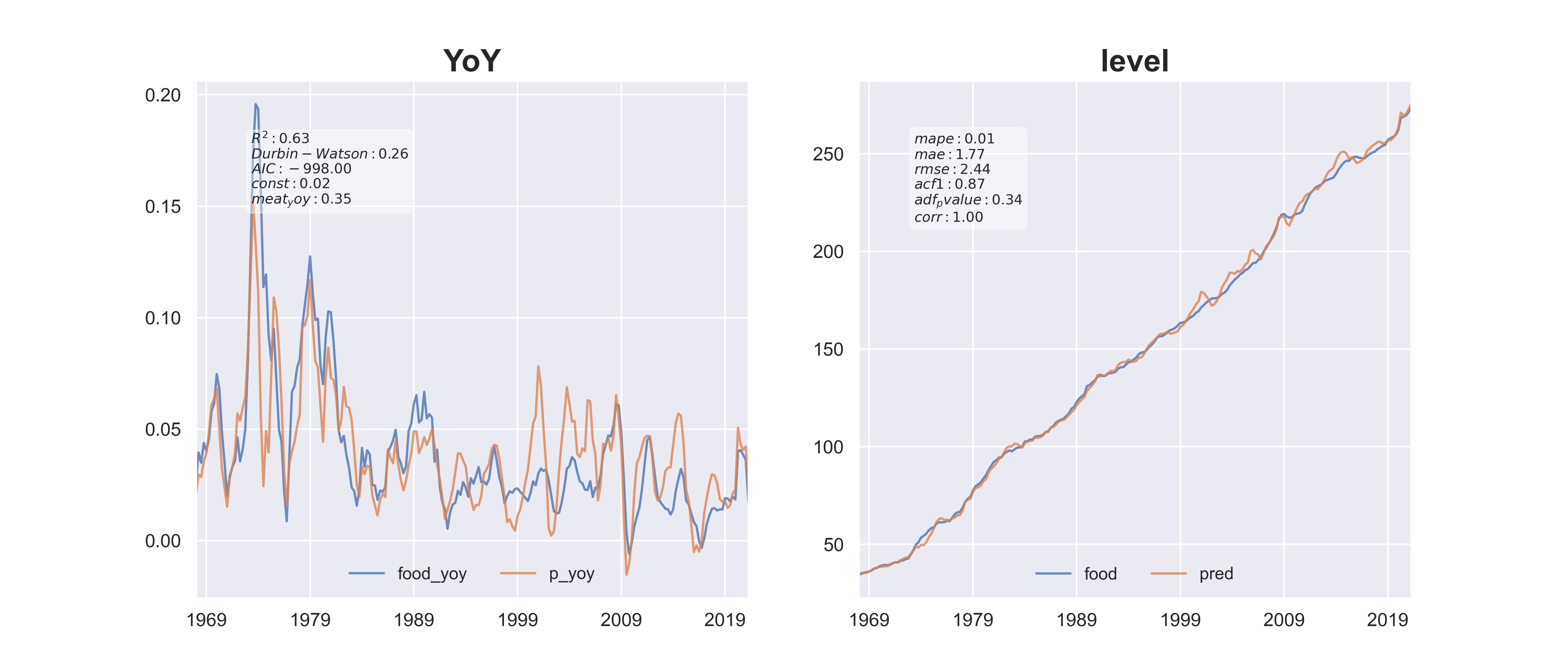
# plot
fig, ax = plt.subplots(1,2, figsize=(14,6))
df[[y,'p_yoy']].plot(ax=ax[0], title='YoY',alpha=.8)
df[['food','pred']].plot(ax=ax[1], title='level', alpha=.8)
w1 = df.index[2] #where to put text
h1 = np.min(df[y]) +0.01
# for YoY performance
textstr0 = '\n'.join((
r'$R^2: %.2f$'%(model.rsquared),
r'$Durbin-Watson: %.2f$'%(dw),
r'$AIC: %.2f$'%(aic),
r'$%s: %.2f$'%(model.params.index[0],model.params[0]),
r'$%s: %.2f$'%(model.params.index[1],model.params[1])
))
# for the level performance
textstr1 = '\n'.join((
r'$mape: %.2f$'%(accuracy_dict['mape']),
r'$mae: %.2f$'%(accuracy_dict['mae']),
r'$rmse: %.2f$'%(accuracy_dict['rmse']),
r'$acf1: %.2f$'%(accuracy_dict['acf1']),
r'$adf_pvalue: %.2f$'%(accuracy_dict['adf_pvalue']),
r'$corr: %.2f$'%(accuracy_dict['corr']),
))
textstr_lt = [textstr0, textstr1]
props = dict(boxstyle='round', facecolor='white',alpha=0.4)
for i in range(2):
ax[1].set_xlabel("")
ax[i].text(.1,.9, textstr_lt[i], fontsize=9, transform=ax[i].transAxes, va='top',bbox=props)
ax[i].legend(loc='lower center',ncol=2, frameon=False)
ARIMA Models
ARIMA Models for the Level Taget
Non-seasonal and non-stationary time series can be modeled using ARIMA. An ARIMA model is characterized by 3 terms:
- p: the order of the AR term (how many lags)
- d: the number of differencing required to make the time series stationary; use acf plot
- q: the order of the MA term
Note that ARIMA model coefficients AR(p) and MA(q) terms are bounded between (−1,1) or else the process is not stationary.
The statsmodels statsmodels.tsa.arima_model.ARIMA has the order of (p,d,q). So the first term in this ARIMA class is order of AR term, then differencing, and finally MA.
PACF (Partial Autocorrelation) plot: used for identify number of AR terms, i.e. number of lags The right order of differencing is the minimum differencing required to get a near-stationary series which roams around a defined mean and the ACF plot reaches to zero fairly quick. Adjusted Box-Tiao (ABT). In ABT, ARIMAX models with AR terms using the Box-Tiao method.
First of all, since P-value is greater than the significance level, we take difference of the series and plot autocorrelation plot. Note that because our data has datetime index, we should not use sharex=True, because datetime index and range index cannot be shared.
from statsmodels.graphics.tsaplots import plot_acf, plot_pacf
from statsmodels.tsa.stattools import adfuller
stationary_result = adfuller(df.food_yoy)
print('ADF Statistic: %f' % stationary_result[0])
print('p-value: %f' % stationary_result[1])
[Out]:
ADF Statistic: -1.780230
p-value: 0.390320
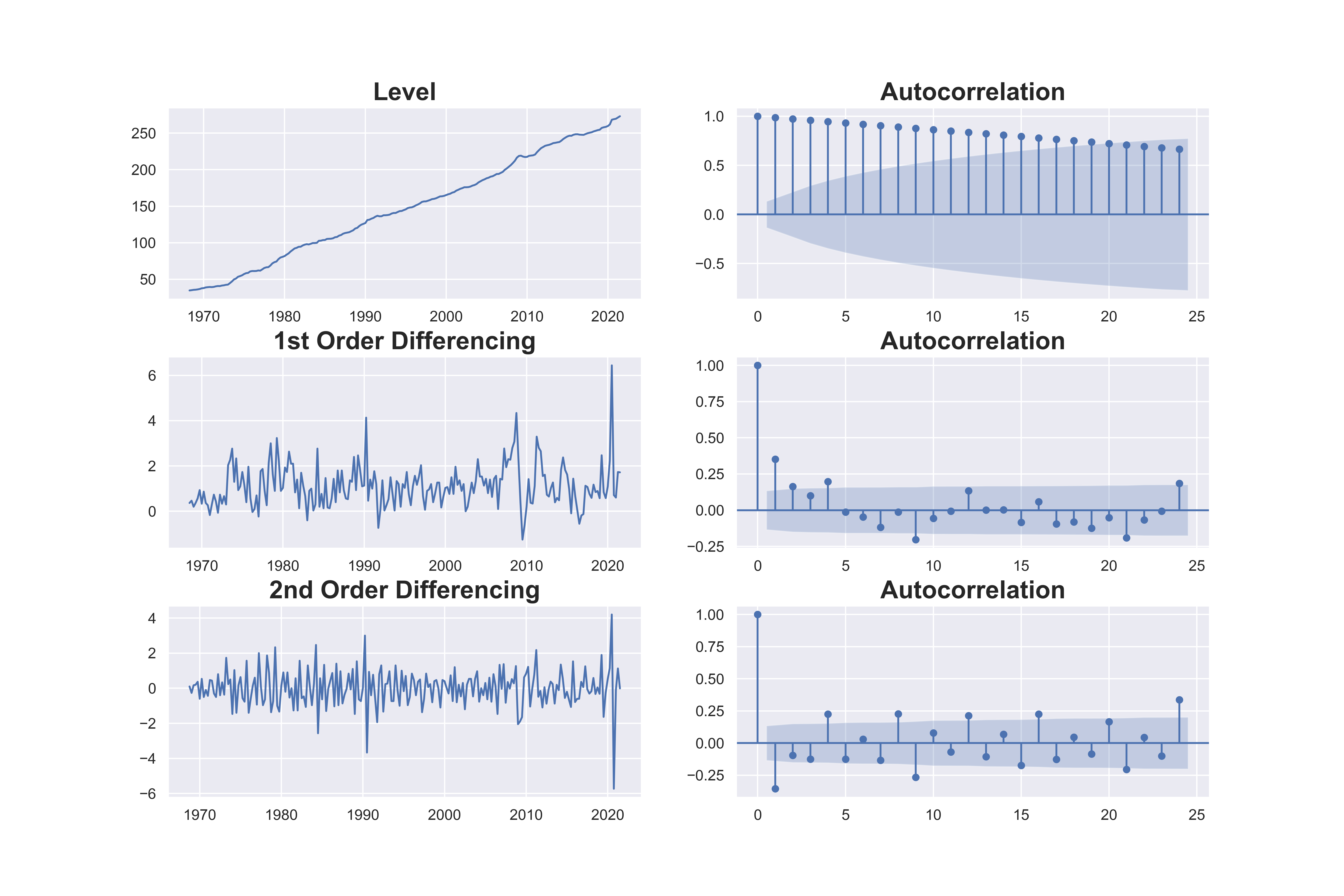
# Original Series
fig, axes = plt.subplots(3, 2,figsize=(15,10) #sharex=False
axes[0, 0].plot(df.food); axes[0, 0].set_title('Level')
plot_acf(df.food, ax=axes[0, 1])
# 1st Differencing
axes[1, 0].plot(df.food.diff()); axes[1, 0].set_title('1st Order Differencing')
plot_acf(df.food.diff().dropna(), ax=axes[1, 1])
# 2nd Differencing
axes[2, 0].plot(df.food.diff().diff()); axes[2, 0].set_title('2nd Order Differencing')
plot_acf(df.food.diff().diff().dropna(), ax=axes[2, 1])
The acf plots show that after the first difference, the autocorrelation has dropped a lot. Although there is still a bit of autocorrelation at lag 1, the first difference is better than the second difference, which went to negative correlation on the first lag. Therefore we will go with AR 1.
from statsmodels.graphics.tsaplots import plot_acf, plot_pacf
from statsmodels.tsa.stattools import adfuller
stationary_result = adfuller(df.food_yoy)
print('ADF Statistic: %f' % stationary_result[0])
print('p-value: %f' % stationary_result[1])
[Out]:
ADF Statistic: -1.780230
p-value: 0.390320
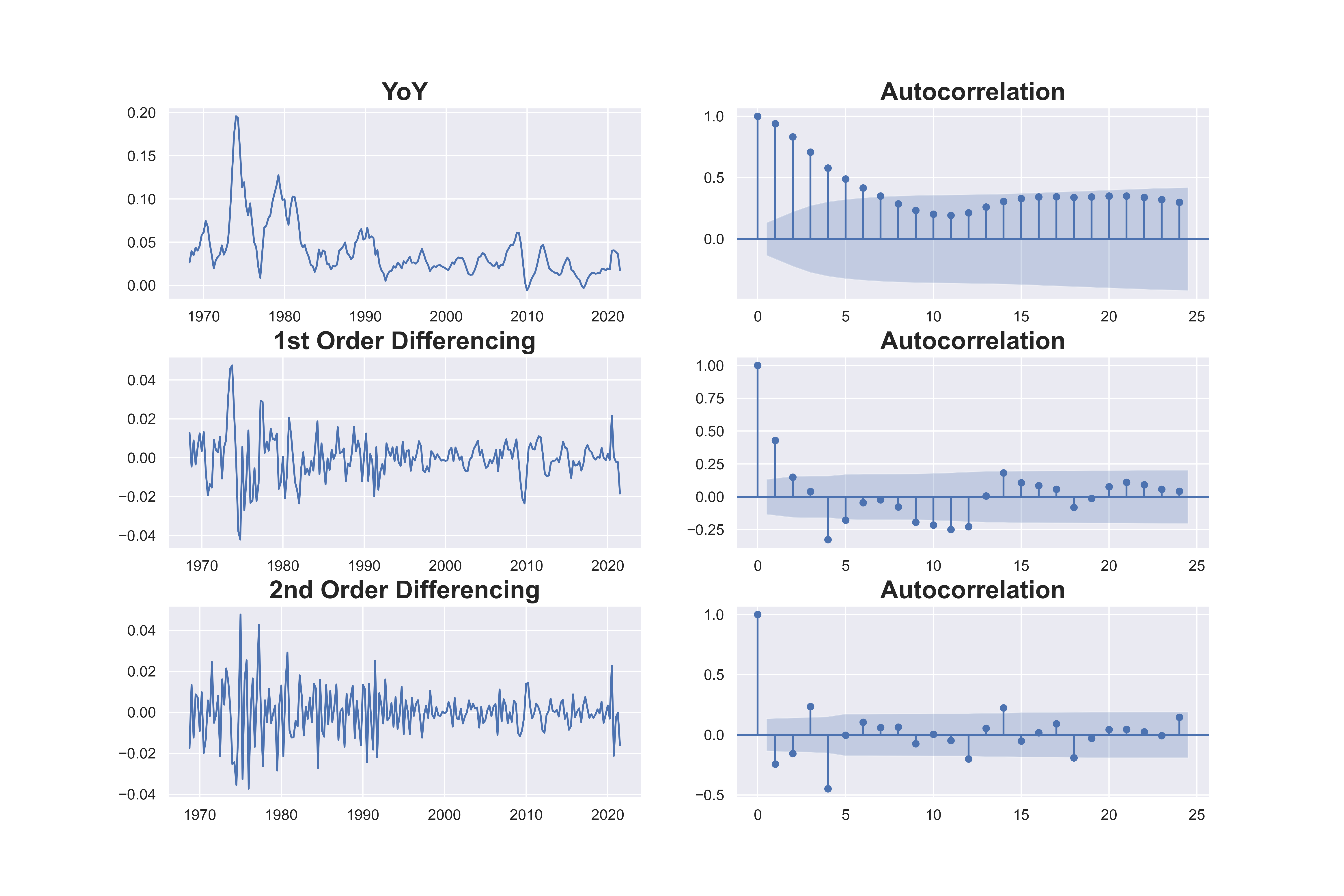
The YoY transformed autocorrelation plot is below. We see that even the YoY transformed price has strong autocorrelation in the first few lags. This is understandable because price increase/decrease don’t just last a quarter, and has momemtum effect. After the first difference, the data looks stationary but still has a little positive serial correlation at lag 1, but not severa. We will go with AR 1 as well. Besides visual examination, we can run some statistical tests as well on the number of differences needed to achieve stationarity.
The pmdarima package provides many convenient methods. Using the ndiffs from pmdarima.arima.utils we see the all three different tests agree on differencing once for food. For the YoY transformation, ADF and KPSS method concludes 1 differencing, but the PP method says no differencing is needed.
from pmdarima.arima.utils import ndiffs
y = df.food
print("ndiff by Adf Test:", ndiffs(y, test='adf'))
print("ndiff by KPSS:", ndiffs(y, test='kpss'))
print("ndiff by PP:",ndiffs(y, test='pp'))
[Out]:
ndiff by Adf Test: 1
ndiff by KPSS: 1
ndiff by PP: 1

y = df.food_yoy
print("ndiff by Adf Test:", ndiffs(y, test='adf'))
print("ndiff by KPSS:", ndiffs(y, test='kpss'))
print("ndiff by PP:",ndiffs(y, test='pp'))
[Out]:
ndiff by Adf Test: 0
ndiff by KPSS: 1
ndiff by PP: 0
We begin with an ARIMA(1,1,1) model. The ma term ma.L1.D.food is not signficant, which is dropped in the second try in an ARIMA(1,1,0) model. We notice that AIC and BIC dropped, and the p-value for ar.L1.D.food is smaller, which means the ARIMA(1,1,0) is a simpler and more robust model than ARIMA(1,1,1).
from statsmodels.tsa.arima_model import ARIMA
train = df.food
model = ARIMA(train, order=(1, 1, 0)).fit()
model.summary()
[Out]:
                            ARIMA Model Results
==============================================================================
Dep. Variable:                 D.food   No. Observations:                  213
Model:                 ARIMA(1, 1, 1)   Log Likelihood                -273.430
Method:                       css-mle   S.D. of innovations              0.873
Date:                Sun, 16 May 2021   AIC                            554.860
Time:                        15:14:31   BIC                            568.305
Sample:                    06-30-1968   HQIC                           560.294
                         - 06-30-2021
================================================================================
                   coef    std err          z      P>|z|      [0.025      0.975]
--------------------------------------------------------------------------------
const            1.1184      0.100     11.197      0.000       0.923       1.314
ar.L1.D.food     0.5186      0.204      2.538      0.011       0.118       0.919
ma.L1.D.food    -0.1932      0.241     -0.802      0.422      -0.665       0.279
                                    Roots
=============================================================================
                  Real          Imaginary           Modulus         Frequency
-----------------------------------------------------------------------------
AR.1            1.9283           +0.0000j            1.9283            0.0000
MA.1            5.1752           +0.0000j            5.1752            0.0000
-----------------------------------------------------------------------------

model = ARIMA(train, order=(1, 1, 0)).fit()
model.summary()
[Out]:
                             ARIMA Model Results
==============================================================================
Dep. Variable:                 D.food   No. Observations:                  213
Model:                 ARIMA(1, 1, 0)   Log Likelihood                -273.749
Method:                       css-mle   S.D. of innovations              0.875
Date:                Sun 16 May 2021    AIC                            553.497
Time:                        15:21:19   BIC                            563.581
Sample:                    06-30-1968   HQIC                           557.572
                         - 06-30-2021
================================================================================
                   coef    std err          z      P>|z|      [0.025      0.975]
--------------------------------------------------------------------------------
const            1.1187      0.092     12.130      0.000       0.938       1.299
ar.L1.D.food     0.3519      0.064      5.491      0.000       0.226       0.477
                                    Roots
=============================================================================
                  Real          Imaginary           Modulus         Frequency
-----------------------------------------------------------------------------
AR.1            2.8419           +0.0000j            2.8419            0.0000
-----------------------------------------------------------------------------
You can find out the required number of AR terms by inspecting the Partial Autocorrelation (PACF) plot.
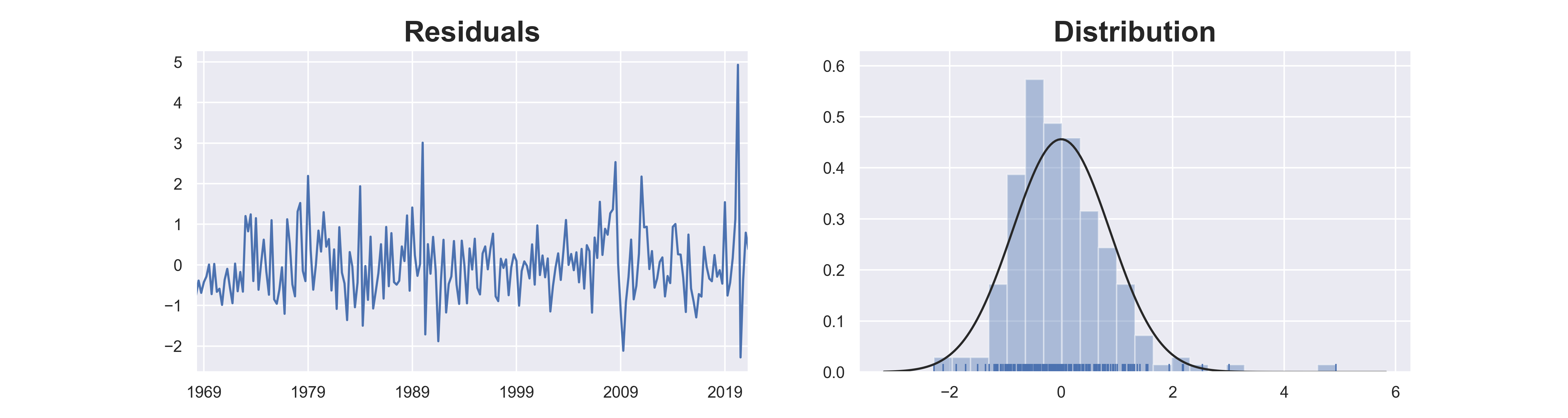
# residual
residuals =model.resid
from scipy import stats
from scipy.stats import norm
norm_test =stats.anderson(residuals, dist='norm')
stat, p = stats.kstest(residuals, 'norm')
print('p-value: {0: .4f}'.format(p))
[Out]:
p-value:  0.0958

fig, ax = plt.subplots(1,2, figsize=(15,4))
residuals.plot(title="Residuals", ax=ax[0])
sns.distplot(residuals, fit=norm, kde=False, rug=True, ax=ax[1])
plt.title("Distribution")
plt.show()
title = "ARIMA(1,1,0) non-dynamic level actual vs predicted"
model.plot_predict(dynamic=False)
The dynamic=False specification in .plot_predict uses the in-sample lagged values for prediction, which can make the predicted look better than they actually are. We will get to out-of-sample testing in the next section.
%20non-dynamic%20level%20actual%20vs%20predicted.png)
YoY ARIMA Models
Both the AR and MA terms are significant.
When we have AR 3, AIC and HQIC increased but BIC dropped slightly. We will go with AR 2 and see how the residual looks like.
from statsmodels.tsa.arima_model import ARIMA
train = df.food_yoy
model = ARIMA(train, order=(2, 1, 0)).fit()
model.summary()
[Out]:
                            ARIMA Model Results
==============================================================================
Dep. Variable:             D.food_yoy   No. Observations:                  213
Model:                 ARIMA(2, 1, 1)   Log Likelihood                 693.187
Method:                       css-mle   S.D. of innovations              0.009
Date:                Mon, 17 May 2021   AIC                          -1376.375
Time:                        18:32:01   BIC                          -1359.569
Sample:                    06-30-1968   HQIC                         -1369.583
                         - 06-30-2021
====================================================================================
                       coef    std err          z      P>|z|      [0.025      0.975]
------------------------------------------------------------------------------------
const            -1.347e-05      0.001     -0.012      0.990      -0.002       0.002
ar.L1.D.food_yoy    -0.3167      0.071     -4.456      0.000      -0.456      -0.177
ar.L2.D.food_yoy     0.1866      0.071      2.635      0.008       0.048       0.325
ma.L1.D.food_yoy     0.9554      0.019     49.319      0.000       0.917       0.993
                                    Roots
=============================================================================
                  Real          Imaginary           Modulus         Frequency
-----------------------------------------------------------------------------
AR.1           -1.6171           +0.0000j            1.6171            0.5000
AR.2            3.3147           +0.0000j            3.3147            0.0000
MA.1           -1.0467           +0.0000j            1.0467            0.5000
-----------------------------------------------------------------------------

title = "ARIMA(2,1,0) YoY actual vs predicted"
model.plot_predict(dynamic=False)
%20YoY%20actual%20vs%20predicted.png)
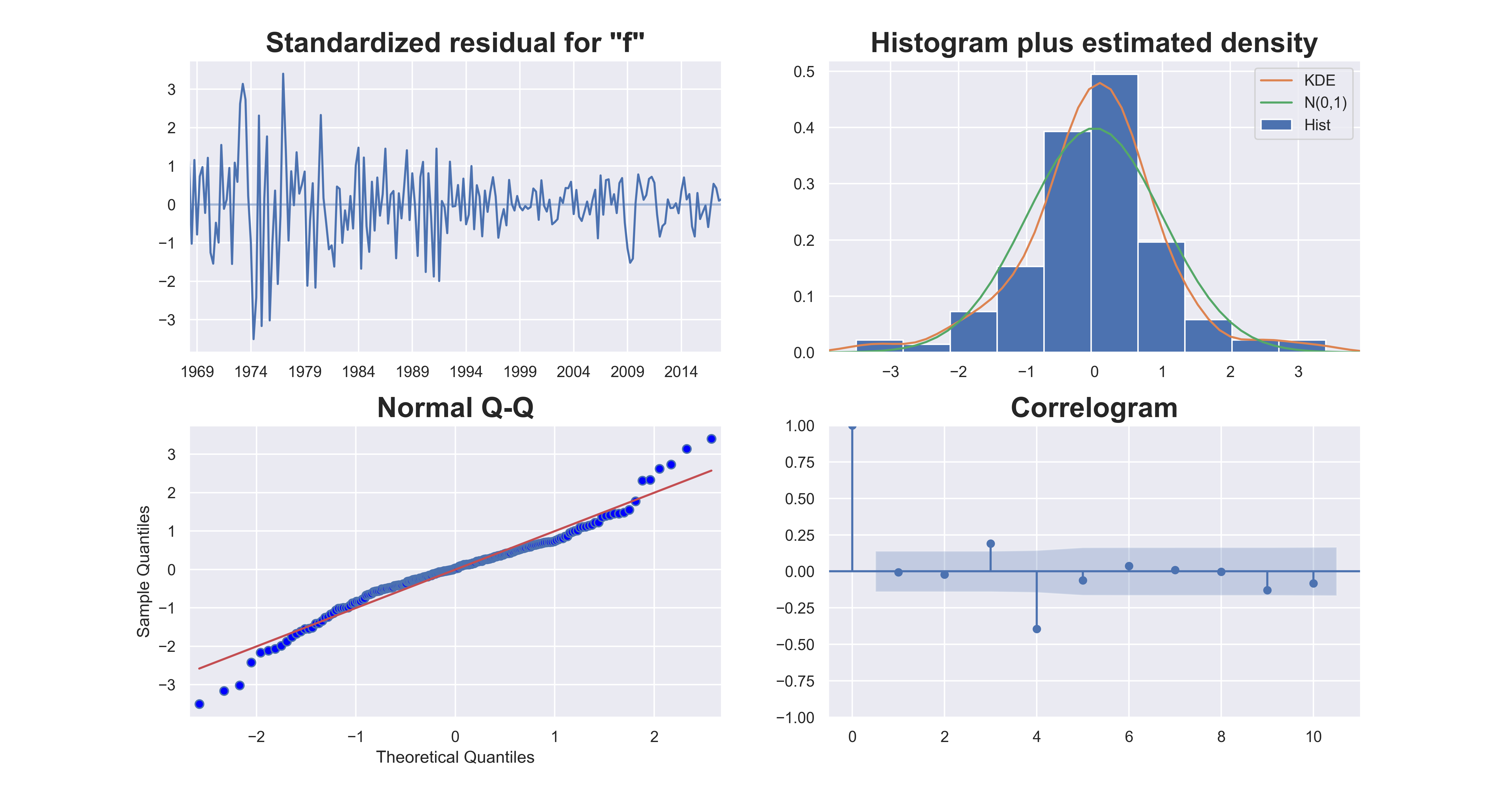
A more convenient way is to use the model.plot_diagnostics() method from statsmodels.
# better way to plot residual diagnostics
model.plot_diagnostics(figsize=(15,8))
plt.subplots_adjust(hspace=0.25)
standardized residual (top left): The residuals seem to fluctuate around a mean of zero but the variance does not look constant. In the period before 1080, the model tends to underpredict, resulting in larger residuals than later period. The residuals in 1990s and the period around and after 2012 are smaller than other time periods. This means that there may be structural changes in the data, and there are external factors should be accounted for, if possible.
Because of the patterns we see in the residual plot, we should run structural break tests on the data. But visually we can already tell there are structural breaks.
Histogram plus estimated density (top right): The standarized residual density is more concentrated in the middle, and does not look standard normal. But it is not too far deviated from it.
Normal Q-Q (bottom left): All the dots should fall perfectly in line with the red line. Any significant deviations would imply the distribution is skewed.
Correlogram (bottom right): The Correlogram, aka, ACF plot shows the residuals are autocorrelated at the 3rd lag (positive) and the 4th lag (negative). Any residual autocorrelation implies that there is some pattern in the data that are not explained by the model. We will need to find out if we can add more inputs and/or explain the discrepancy if we accept the limitation.
Model Evaluation 3: Out of Sample Testings
We have so far worked without any validation, which is certainly wrong. But we did that to focus on illustrating the individual pieces. When prediction/forecast is the goal, out of sample testing is essential for model performance evaluation.
One-Time Train/Test Split
Now, we will incorpate out of sample validation in model building.
from statsmodels.tsa.arima.model import ARIMA
# train/test
train = df.food[:200]
test = df.food[200:] # 14 records
model = ARIMA(train, order=(1, 1, 0)).fit()
# Forecast
fc= model.forecast(14, alpha=0.05) # 95% conf
forecast = model.get_forecast(14)
yhat = forecast.predicted_mean
yhat_conf_int = forecast.conf_int(alpha=0.05)
test_pred = test.to_frame().join([fc,yhat_conf_int])
title = "ARIMA Forecast (level)"
test_pred.plot()
plt.plot(train, label='training')
plt.fill_between(test.index, test_pred['lower food'], test_pred['upper food'],
color='k', alpha=.15)
plt.legend(frameon=False, loc='lower center', ncol=4)
# plot test data and forecast together with training data
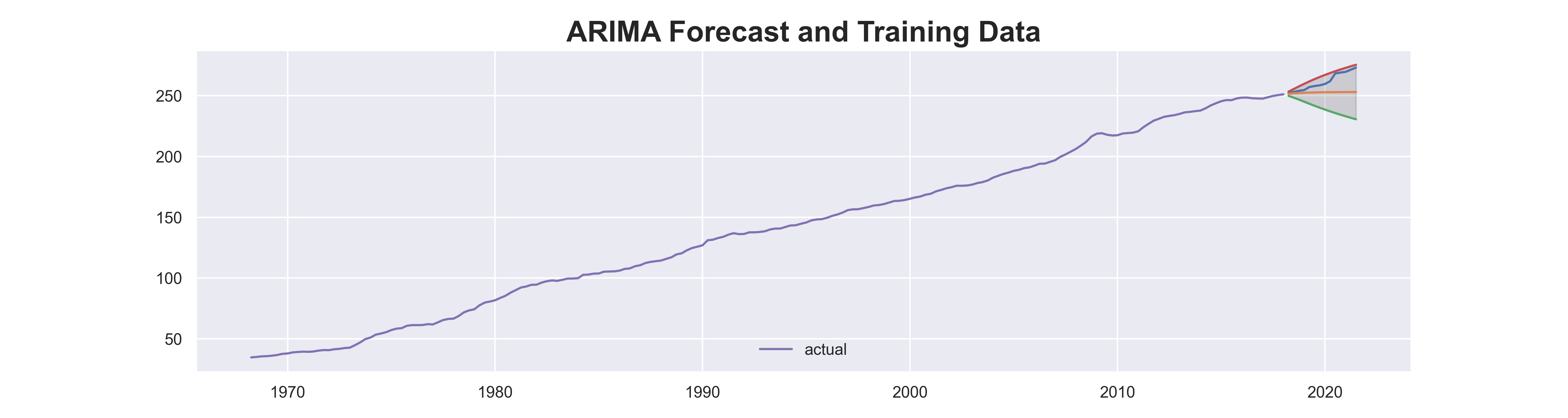
title ="ARIMA Forecast and Training Data"
plt.plot(test_pred)
plt.fill_between(test.index, test_pred['lower food'], test_pred['upper food'],
color='k', alpha=.15)
plt.plot(train,label='actual')
Using out-of-sample testing, we see that the forecast result is not good as it did not actually capture the upward trend. The actual food price is close to the 95% upper bound.
.png)
The forecast quality is bad.
Below is a snippet for the YoY out of sample testing.
# yoy
title = "ARIMA Forecast (yoy)"
train = df.food_yoy[:200]
test = df.food_yoy[200:]
model = ARIMA(train, order=(2, 1, 0)).fit()
# Forecast
fc= model.forecast(14, alpha=0.05) # 95% conf
forecast = model.get_forecast(14)
yhat = forecast.predicted_mean
yhat_conf_int = forecast.conf_int(alpha=0.05)
test_pred = test.to_frame().join([fc,yhat_conf_int])
test_pred.plot()
# plot test data and forecast together with training data
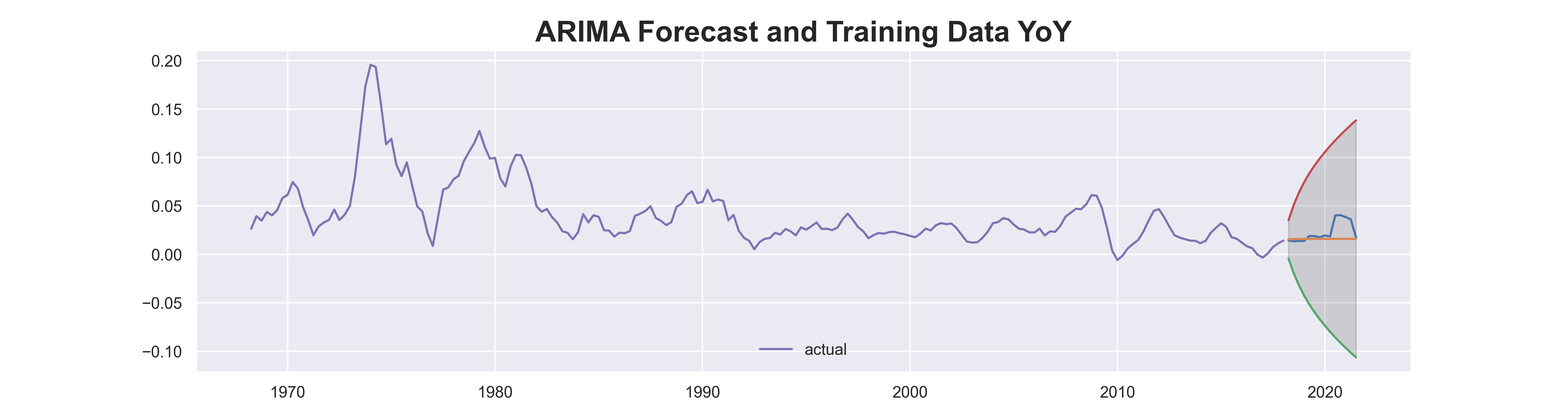
title ="ARIMA Forecast and Training Data YoY"
plt.plot(test_pred)
plt.fill_between(test.index, test_pred['lower food_yoy'], test_pred['upper food_yoy'],
color='k', alpha=.15)
plt.plot(train,label='actual')
plt.legend(frameon=False, loc='lower center', ncol=4)
accuracy_dict = accuracy_dict_function(test_pred.predicted_mean,test_pred.food_yoy)
accuracy_dict
[Out]:
{'mape': 0.26,
'me': -0.01,
'mae': 0.01,
'mpe': -0.19,
'rmse': 0.01,
'acf1': 0.67,
'adf_pvalue': 0.08,
'corr': 0.34}
We skip the first plot and look at the second plot with training data. The same problem with the level forecast shows in the YoY forecast as well. The forecasts completely misses the rising trend in the last few quarters. This is understandable, because our world just got shocked by Covid-19, which is completely an unexpected systematic stress that is not related to lags.
ARMA model is not suitable for stress testing.
Automatic ARIMA
It is not feasible for us to manually check each iteration for every model. So we will need an automated process for selecting the best model. See Tips to using auto_arima for the nuances for the hyper parameters.
There are two ways to run the automated procedure: stepwise and parallelized. The parallel approach is a naive, brute force grid search over all combinations of hyper parameters as specified. Because of its grid search nature, it can take longer time.
Here is from the documentation:
The auto-ARIMA process seeks to identify the most optimal parameters for an ARIMA model, settling on a single fitted ARIMA model. This process is based on the commonly-used R function,forecast::auto.arima.
Auto-ARIMA works by conducting differencing tests (i.e.,Kwiatkowski–Phillips–Schmidt–Shin, Augmented Dickey-Fuller orPhillips–Perron) to determine the order of differencing, d, and thenfitting models within ranges of defined start_p, max_p,start_q, max_q ranges. If the seasonal optional is enabled,auto-ARIMA also seeks to identify the optimal P and Q hyper-parameters after conducting the Canova-Hansen to determine the optimal order of seasonal differencing, D.
In order to find the best model, auto-ARIMA optimizes for a giveninformation_criterion, one of (‘aic’, ‘aicc’, ‘bic’, ‘hqic’, ‘oob’)(Akaike Information Criterion, Corrected Akaike Information Criterion,Bayesian Information Criterion, Hannan-Quinn Information Criterion, or”out of bag”–for validation scoring–respectively) and returns the ARIMAwhich minimizes the value.
Note that due to stationarity issues, auto-ARIMA might not find a suitable model that will converge. If this is the case, a ValueError will be thrown suggesting stationarity-inducing measures be taken priorto re-fitting or that a new range of order values be selected. Non-stepwise (i.e., essentially a grid search) selection can be slow,especially for seasonal data. Stepwise algorithm is outlined in Hyndman and Khandakar (2008)
model = pm.auto_arima(train.values, start_p=1, start_q=1,
                      test='adf',       # use adftest to find optimal 'd'
                      max_p=3, max_q=3, # p=AR order, q = MA order)
                      m=1,              # frequency of series
                      d=None,           # let model determine number of differencing
                      seasonal=False,   # No Seasonality
                      start_P=0,
                      D=0,
                      trace=True,
                      error_action='ignore',
                      suppress_warnings=True,
                      stepwise=True)

model.summary()

Performing stepwise search to minimize aic
 ARIMA(1,0,1)(0,0,0)[0]             : AIC=-1272.709, Time=0.21 sec
 ARIMA(0,0,0)(0,0,0)[0]             : AIC=-606.610, Time=0.02 sec
 ARIMA(1,0,0)(0,0,0)[0]             : AIC=-1221.578, Time=0.02 sec
 ARIMA(0,0,1)(0,0,0)[0]             : AIC=-867.145, Time=0.08 sec
 ARIMA(2,0,1)(0,0,0)[0]             : AIC=-1264.990, Time=0.07 sec
 ARIMA(1,0,2)(0,0,0)[0]             : AIC=-1278.801, Time=0.25 sec
 ARIMA(0,0,2)(0,0,0)[0]             : AIC=-1021.603, Time=0.18 sec
 ARIMA(2,0,2)(0,0,0)[0]             : AIC=-1263.891, Time=0.12 sec
 ARIMA(1,0,3)(0,0,0)[0]             : AIC=-1337.314, Time=0.38 sec
 ARIMA(0,0,3)(0,0,0)[0]             : AIC=-1115.481, Time=0.23 sec
 ARIMA(2,0,3)(0,0,0)[0]             : AIC=-1327.319, Time=0.48 sec
 ARIMA(1,0,3)(0,0,0)[0] intercept   : AIC=-1348.572, Time=0.52 sec
 ARIMA(0,0,3)(0,0,0)[0] intercept   : AIC=inf, Time=0.60 sec
 ARIMA(1,0,2)(0,0,0)[0] intercept   : AIC=-1283.426, Time=0.43 sec
 ARIMA(2,0,3)(0,0,0)[0] intercept   : AIC=-1343.695, Time=0.58 sec
 ARIMA(0,0,2)(0,0,0)[0] intercept   : AIC=-1145.968, Time=0.38 sec
 ARIMA(2,0,2)(0,0,0)[0] intercept   : AIC=-1274.859, Time=0.53 sec

Best model:  ARIMA(1,0,3)(0,0,0)[0] intercept
Total fit time: 5.116 seconds
                               SARIMAX Results
==============================================================================
Dep. Variable:                      y   No. Observations:                  200
Model:               SARIMAX(1, 0, 3)   Log Likelihood                 680.286
Date:                Wed, 19 May 2021   AIC                          -1348.572
Time:                        10:25:43   BIC                          -1328.782
Sample:                             0   HQIC                         -1340.563
                                - 200
Covariance Type:                  opg
==============================================================================
                 coef    std err          z      P>|z|      [0.025      0.975]
------------------------------------------------------------------------------
intercept      0.0148      0.004      3.630      0.000       0.007       0.023
ar.L1          0.6647      0.047     14.212      0.000       0.573       0.756
ma.L1          0.8489      0.053     16.156      0.000       0.746       0.952
ma.L2          0.8115      0.049     16.617      0.000       0.716       0.907
ma.L3          0.8911      0.054     16.511      0.000       0.785       0.997
sigma2      6.738e-05    5.7e-06     11.817      0.000    5.62e-05    7.86e-05
===================================================================================
Ljung-Box (L1) (Q):                   0.26   Jarque-Bera (JB):               108.74
Prob(Q):                              0.61   Prob(JB):                         0.00
Heteroskedasticity (H):               0.14   Skew:                             1.06
Prob(H) (two-sided):                  0.00   Kurtosis:                         5.92
===================================================================================
The automated procedure shows that ARIMA(1,0,3) is the best model, with 1 lag and 3 MA terms.
Using Auto-ARIMA to Forecast
Fit an ARIMA to a vector, y, of observations with an optional matrix of exogenous variables, and then generate predictions.
Parameters
y : The time-series to which to fit the ARIMA estimator. This mayeither be a Pandas Series object or a numpy array. This should be a one-dimensional array of floats, and should not contain anynp.nan or np.inf values.
X : An optional 2-d array of exogenous variables. If provided, these variables are used as additional features in the regression operation. This should not include a constant or trend.
n_periods : (default=10) The number of periods in the future to forecast.
Automated ARIMA
import pmdarima as pm
model = pm.auto_arima(train.values, start_p=1, start_q=1,
test='adf', # use adftest to find optimal 'd'
max_p=3, max_q=3, # maximum p and q
m=4, # frequency of series, period for seasonal differencing
d=None, # let model determine 'd'
seasonal=False, # No Seasonality
start_P=0,
D=0,
trace=True,
error_action='ignore',
suppress_warnings=True,
stepwise=True)
model.summary()
pred = model.fit_predict(train, n_periods=len(test))
pred_s = pd.Series(pred, index=test.index)
pred_s.name='pred'
test.to_frame().join(pred_s).plot()
# Forecast
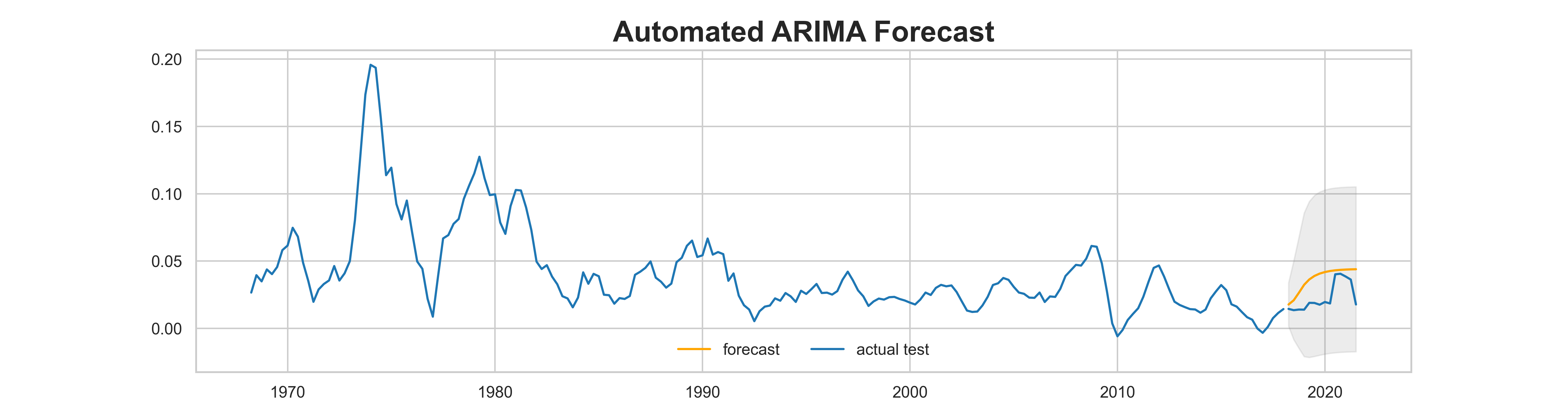
title = "Automated ARIMA Forecast"
n_periods = len(test)
fc, confint = model.fit_predict(train, n_periods=n_periods, return_conf_int=True) # train is 1 dim
fc_idx = test.index
# for plotting
fc_series = pd.Series(fc, index=fc_idx)
low = pd.Series(confint[:, 0], index=fc_idx)
high = pd.Series(confint[:, 1], index=fc_idx)
# Plot
sns.set_style('white')
plt.plot(train, color=blue)
plt.plot(fc_series, color='orange', label='forecast')
plt.plot(test, color=blue, label='actual test')
plt.fill_between(low.index,
low,
high,
color='grey', alpha=.15)
The result looks better than the one manually created.
ARIMAX with X (exogenous)
Let’s pretend that meat prices drive food prices. The downside is that in order to make predictions for food_yoy, we will need the forecast for meat_yoy.
import pmdarima as pm
# train, X=df.meat_yoy[:200].to_frame() will also work, as long as they have the same index
model = pm.auto_arima(train.values, X=df.meat_yoy[:200].values.reshape(-1,1) ,start_p=1, start_q=1,
test='adf', # use adftest to find optimal 'd'
max_p=3, max_q=3, # maximum p and q
m=4, # frequency of series, period for seasonal differencing
d=None, # let model determine 'd'
seasonal=False, # No Seasonality
start_P=0,
D=0,
trace=True,
error_action='ignore',
suppress_warnings=True,
stepwise=True)
[Out]:
Performing stepwise search to minimize aic
ARIMA(1,0,1)(0,0,0)[0] : AIC=-1406.458, Time=0.42 sec
ARIMA(0,0,0)(0,0,0)[0] : AIC=-799.668, Time=0.05 sec
ARIMA(1,0,0)(0,0,0)[0] : AIC=-1365.289, Time=0.16 sec
ARIMA(0,0,1)(0,0,0)[0] : AIC=-1032.365, Time=0.11 sec
ARIMA(2,0,1)(0,0,0)[0] : AIC=-1422.762, Time=0.37 sec
ARIMA(2,0,0)(0,0,0)[0] : AIC=-1420.931, Time=0.29 sec
ARIMA(3,0,1)(0,0,0)[0] : AIC=-1427.298, Time=0.48 sec
ARIMA(3,0,0)(0,0,0)[0] : AIC=-1422.412, Time=0.39 sec
ARIMA(3,0,2)(0,0,0)[0] : AIC=-1409.680, Time=0.73 sec
ARIMA(2,0,2)(0,0,0)[0] : AIC=-1425.466, Time=0.37 sec
ARIMA(3,0,1)(0,0,0)[0] intercept : AIC=-1424.524, Time=0.57 sec
Best model: ARIMA(3,0,1)(0,0,0)[0]
model.summary()
[Out]:
SARIMAX Results
==============================================================================
Dep. Variable: y No. Observations: 200
Model: SARIMAX(3, 0, 1) Log Likelihood 719.649
Date: Wed, 19 May 2021 AIC -1427.298
Time: 17:59:28 BIC -1407.508
Sample: 0 HQIC -1419.289
- 200
Covariance Type: opg
==============================================================================
coef std err z P>|z| [0.025 0.975]
------------------------------------------------------------------------------
x1 0.2302 0.011 21.677 0.000 0.209 0.251
ar.L1 0.6662 0.085 7.817 0.000 0.499 0.833
ar.L2 0.5983 0.126 4.732 0.000 0.350 0.846
ar.L3 -0.2915 0.066 -4.398 0.000 -0.421 -0.162
ma.L1 0.9110 0.055 16.435 0.000 0.802 1.020
sigma2 4.259e-05 3.55e-06 12.005 0.000 3.56e-05 4.95e-05
===================================================================================
Ljung-Box (L1) (Q): 1.26 Jarque-Bera (JB): 32.33
Prob(Q): 0.26 Prob(JB): 0.00
Heteroskedasticity (H): 0.17 Skew: -0.01
Prob(H) (two-sided): 0.00 Kurtosis: 4.97
# model.predict(n_periods=10, X=None, return_conf_int=False, alpha=0.05, **kwargs)
pred = model.predict(n_periods=14, X=df.meat_yoy[200:].to_frame())
pred_s = pd.Series(pred, index=test.index)
pred_s.name='pred'
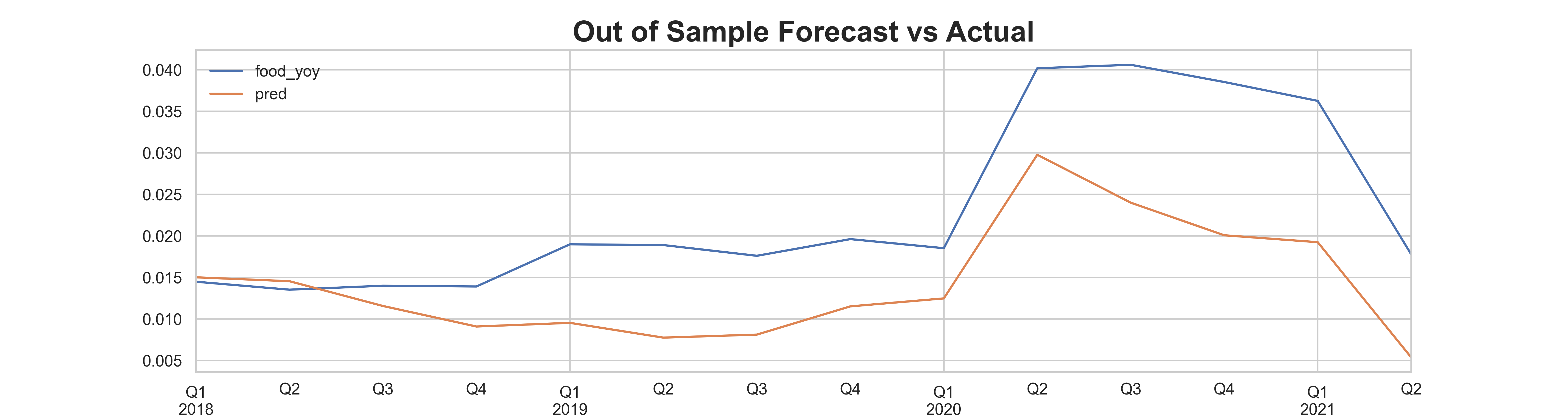
title = "Out of Sample Forecast vs Actual"
test.to_frame().join(pred_s).plot()
We see that the result is a lot better. This is because we have the actual meat data for the forecast period. This is in fact “cheating”. Because in reality, we do not know what meat prices are in the future. We will need to develope a model to forecast meat prices before using the ARIMAX model.
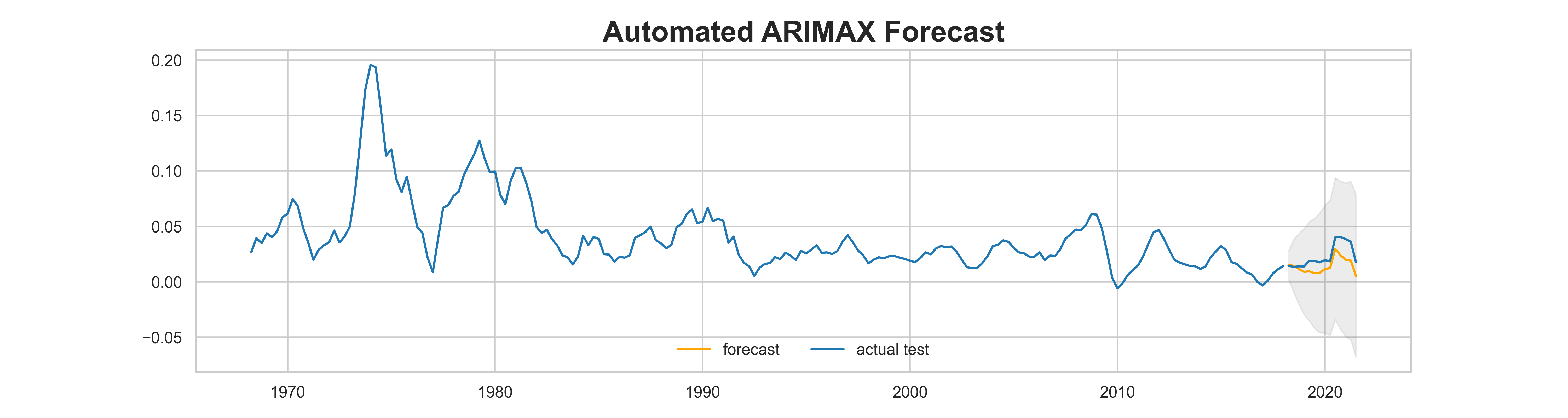
title = "Automated ARIMAX Forecast"
n_periods = len(test)
fc, confint = fc, confint = model.predict(n_periods=n_periods,
                                  exogenous=df.meat_yoy[200:].to_frame(),
                                  return_conf_int=True)
fc_idx = test.index
fc_series = pd.Series(fc, index=fc_idx)
low = pd.Series(confint[:, 0], index=fc_idx)
high = pd.Series(confint[:, 1], index=fc_idx)
# Plot
sns.set_style('whitegrid')
plt.plot(train, color=blue)
plt.plot(fc_series, color='orange', label='forecast')
plt.plot(test, color=blue, label='actual test')
plt.fill_between(low.index,
                 low,
                 high,
                 color='grey', alpha=.15)
Model Evaluation: Walk Forward Expanding Window Train Test
The purpose of out of sample test/validation is to evaluate model specification and the robustness in predictions. There are different schemes for splitting up the time-indexed data for train and test.

n_train = 195
n_records = df.shape[0]
accuracy_lt =[]
for i in range(n_train, n_records-14):
	train, test = df.food_yoy[0:i], df.food_yoy[i:i+14]
	# print('train=%d, test=%d' % (len(train), len(test)))
    exogenous_train  = df.meat_yoy[0:i].to_frame()
    exogenous_test = df.meat_yoy[i:i+14].to_frame()
    # print("test", test.shape)
    # print("exogenous_train",exogenous_train.shape)
    # print("exogenous_test",exogenous_test.shape)
    # print("train", train.shape)
    axmodel = pm.auto_arima(train, exogenous=exogenous_train,
                           start_p=1, start_q=1,
                           test='adf',
                           max_p=3, max_q=3, m=12,
                           start_P=0, seasonal=False,
                           d=None, D=1, trace=True,
                           error_action='ignore',
                           suppress_warnings=True,
                           stepwise=True)
    print("i = ", i)
    print(axmodel.summary())
    fc, conf_int = model.predict(n_periods=14, X = exogenous_test, return_conf_int=True, alpha=0.05)
    fc_s = pd.Series(fc, index=test.index)
    fc_s.name='fc'
    conf_int_df = pd.DataFrame(conf_int, index=test.index, columns=['lower food_yoy','upper food_yoy' ])
    test_pred = test.to_frame().join([fc_s,conf_int_df])
    accuracy_dict = accuracy_dict_function(test_pred.fc,test_pred.food_yoy)
    # test_pred.plot()
    # plt.fill_between(test.index, test_pred['lower food_yoy'], test_pred['upper food_yoy'],
    #                  color='k', alpha=.15)
    # plt.legend(frameon=False, loc='lower center', ncol=4)
    # plt.show()
    accuracy_lt.append(accuracy_dict)
accuracy_df = pd.DataFrame(accuracy_lt)
accuracy_df
[Out]:
#    mape     me   mae    mpe  rmse  acf1  adf_pvalue  corr
# 0 0.350 -0.000 0.000 -0.220 0.010 0.810       0.990 0.740
# 1 0.400 -0.010 0.010 -0.180 0.010 0.700       1.000 0.840
# 2 0.310 -0.010 0.010 -0.300 0.010 0.670       0.940 0.850
# 3 0.310 -0.010 0.010 -0.300 0.010 0.710       0.130 0.830
# 4 0.340 -0.010 0.010 -0.320 0.010 0.750       0.000 0.830