What is counterparty credit risk

Credit risk from settlement

Settlement exposure

Trading

Payment comes after we agree the price.

Pre-settlement exposure

Derivative. The counterparty defaults, and owes the bank (us) money from derivatives.

Client is obligated to give us 100 MM pounds, we are obligated to give

In reality, the hedge is not a CP. It is my entire book of

To hedge each CP is inefficient.

Suppose sometime during the 6 months, client goes bankcrupt. What happens if fugure forward price is higher, lower?

If we have lots of lots deals, we will talk about netting agreements. In this case, we have only 1.

We are long pounds. The client short. Even though we have not received the pound, we are still long, due to the signed contract.

We will lose a lot more mone if pound goes up since we hedge the position with another CP.

CVA

Expected credit loss due to CP default.

Right way and wrong way

They sell their products into the U.S.. The pricing is almost always in USD. The exporters face currency risk in receivables. The risk to the exporters is the risk that dollar goes down.

Most exporters look at receivables that they sign the contract and the receivalbles for future. They often hedge forecast revenues. Most of the time, they are very good at forecasting their revenue.

But it will make a difference if wrong or

Is the client hedging their forecasted risk or

The forecast may not happen.

I expect to receive dollar 3 months from now, Sell dollar forward.

If the dollar goes up, the client cannot keep the dollar. It has to .

The question is: where is the dollar from the client from? If the dollar is from actual business benefits, then it is fine.

But if the client cannot realize the forecasted revenue, and dollar goes up, this is wrong way risk.

Some have CPR from their business instinct. If dollar goes up by less than 7% it is right way, but when it goes up more than 7% then it is wrong way.

Transforming data to report

Data: spot curves and option prices

Forulas with explicit and implicit assumptions

Discount factors and forward rates

FMV, CVA, DV01, VAR, SVAR, PSE, PSLE

Market risk vs counterparty credit of risk

I think I come up with this phrase “counterparty credit of risk”. As someone who has worked in both insurance and banking, it is clear to me that most risks (or risky assets) are themselves products created to mitigate risks. For example, derivatives are tools that can be used to hedge risks, but they themselves can carry a lot of risk. Buying and selling derivatives is a counterparty credit of risk.

Interestingly, the prices of each of the instruments = cost (to hedge) + some profit, whether for derivatives, forwards, futures,

This is extremely similar to actuarial pricing: insurance price = loss cost + expenses + profit.

Banks are more exposed if they are heavily involved in investing in capital counterparty credits or sales and trading of financial instruments. If a bank has a large trading department, and/or is a big counterparty credit maker, then it will sustantial counterparty credit risk. There are four main types of counterparty credit risk:

1. Interest rate risk: affecting bonds, swaps and other interest rate derivatives.
2. Equity risk (stock counterparty credit risk)
3. Commodity risk: commodity investments and derivatives.
4. FX risk: currency swaps, or investments in currencies.

Most stock and commodity prices, exchange rates and interest rates are provided and updated in real time. But what causes rates and prices to fluctuate a lot? There can be many reasons: economy, political, government policy, operational, industry change, competitions, and many more. Most of them are very difficult or impossible to predict. Let’s keep that in the back of the mind when we think about counterparty credit risk.

1. Interest risk

Interest risk is no stranger to actuaries, who studied theory of interest extensively at the start of the career path.

• DV01: dV/di

commodity: like interest rate swaps, there are commodity “swaps” too. For example, A may want to buy oil at a certain fixed rate, whereas B wants it at floating rate. This creates a situation for commodity swaps.

time horizon	instrument used for hedging	why
short term	futures	cheap and liquid
long term	OTC	because futures are not available for time too far away

Measuring market risk

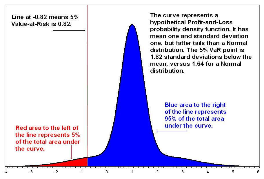
A commonly measure VaR or Value at Risk. is informally defined as:

For a given portfolio, time horizon, and probability p, VaR can be defined informally as the maximum possible loss during that time horizon after we exclude all worse outcomes whose combined probability is at most p.

Daily Value at Risk (DVaR): maximum loss over 1 day to 99% confidence (2.3263 standard deviation). Expected shortfaull: maximum loss over 1 day outside 99% confidence. 3W: average of the three worst-loss paths in a Monte Carlo distribution.

A 1-day 99% Var is the 1-day maximum possible loss at >=99% probability. Informally, it is a hypothetical number that we are very sure that our 1-day loss won’t go above. Our guess would have to be higher if we wanted to be even more sure.

This assumes mark-to-market pricing, and no trading in the portfolio.

But the assumptions are not valid:

• mark-to-market pricing - It is not difficult to obtain mark-to-market prices for the past, but it is impossible to measure mark-to-market pricing for the future. So banks often use book value. This is a proxy but can be very far off.
• no trading in the portfolio. - For institutions, especially the larger ones, their portfolio change often.

VaR can still provide us with some ballpark for our market risk in a “normal day”. However, normal days don’t last.

We have concluded that for various reasons it is close to impossible to predict market risk VaR.

Let’s see how banks and other financial institutions achive the ‘mission impossible’:

Note: Many institutions often first compute 1-day VaR and then scale it up to 10-day VaR using the so-called "square root of time rule". The jargon of "square of time" is nothing but the basic statistics that variance of a sum of n iid random variables is the variance of one of them multipled by the square root of n. This assumption of iid ignores correlation and autocorrelation and assumes constant variance. Obvious not correct! See a simple explaination in Bionic Turtle and Converting 1-Day Volatility to h-Day is Worse than You Think

Regulated financial institutions only have to prove that they are conservative to the regulators.

Since the square root of time rule has been shown empirically to be conservative, and it is simple and straighforward for regulators to manage, it is accepted.

Below are the three most commonly used VaR calcuation methods.

Parametric VaR

• Advantage: easy and fast to compute. All you need is volatility and correlation.
• Diadvantage: it is based on normal assumptions.

Garch VaR

Monte Carlo Simulation

Monte Carlos simply means make some assumption, and simulate based on the assumptions. For example, assume normal distribution of returns with mean of x and standard deviation of y.

Advantage: can build in more flexible distribution assumptions including fat-tails; actual data not required. Disadvantage: computationally intensive, and subject to model risk.

Normal curve:

• start with standard deviations, e.g., running from -6 to 6.
• use small increments, e.g., 0.1, or 0.01.
• In Excel, the curve can be can be calculated using a function: Norm.S.Dist(Z, False)
  • Z is the number of standard deviations
  • False tells the function we want is the “probability density function”
  • True tells that we want cumulative probability or confidence level.

Historical simulations

Advantage: based on actual data, faster than Monte Carlo. Diadvantage: some past data may not be relevant.

Some people strongly believe that what’s coming has never been seen before. They feel much more comfortable using parameters to describe the distribution rather than historical data.

VaR calculation

Assume we own an asset (long position),we lose money when its price falls. “99% confidence” means a fall of 2.3263 standard deviations (in a standard normal distribution).
Our loss depends on

• the volatility of the asset
• the holding period: how long it takes to unwind our trade Against a long position in an asset with spot price S and volatility sigma over time measured in years t: VaR = S - Sexp(-2.3263sigma*square root of t)

VaR diagram

Comparison with Loan Credit Risk

Credit risk: When banks lend out loans, the principals are in the borrower’s hands. The risk is in the borrower may not pay back the loan (in full). In addition, some borrowers may pay back early, which result in interest loss.

Whereas market risk is not funded. The risk is in the loss of the market values of the financial assets.

Comparison with counterparty Credit Risk

Counterparty credit risk arises when it is in the money for the bank because the other party may not keep its promise. Counterparty credit is not a funded risk. The risk is when the contract is “in the money” for the bank, i.e. the risk is only when you have something to lose. At the initation of a contract, neither party owes anything to the other. But as time goes on, the pendulum will be either be favorable to one side or the other. There are two time periods that credit risk can happen:

1. Between margin call (beginning time of having something to lose) and time that the contract must be closed due to counterparty default. This time period is one or two days
2. Between the time of closing contract to the counterparty to the unwinding of the contract (either to find another counterparty or to take over the entire contract). This time period is unknown. This is similar to workout period in credit risk loss given default calculation. The workout period is unknown before it actually happens.

Like market risk, counterpary credit risk also uses simulation to generate loss distributions: simulation => loss distribution. A very similar concept to VaR is PFE, which is the 95th or other higher percentile loss.

Case study

Washington Mutual (WaMu)

Washington Mutual was incorporated on September 25, 1889, after the Great Seattle Fire destroyed 120 acres of the central business district of Seattle. The newly formed company made its first home mortgage loan on the West Coast on February 10, 1890.

By means of serial acquisitions, WaMu expanded its “community-focused” business across most of the western U.S., through the 1980’s and 1990’s. During this period, the Fed Funds rate went from over 19% (Jan, 1981) to below 10%.

Beginning in the 1990’s, WaMu joined the mortage industry in building a presence in subprime lending. During the 1990’s, the Fed Funds rate went from above 8% to below 3% (1993), and then gradually back up to over 5%.

After the dot com crash, the Fed lowered rates, and it bottomed at 2003 with a local minimum of 0.98% on December 2003. The Fed begain raising rates from 2004.

Of course, the year 2003, when interest rate bottomed, was the year the WaMu had a great profitable year. According its 2003 Annual Report

“The end of 2003 brought to a close another successful year for Washington Mutual. Throughout the year, we continued to profitably expand our key businesses nationally and enhance the value of our leading franchise. In addition to reporting record earnings of $3.9 billion, or $4.21 per diluted share, up 5 percent from 2002, we achieved double-digit growth in consumer and mortgage lending, checking accounts, depositor and other retail banking fees and multi-family lending — all primary drivers of our business. And we continued to see marked improvement in our credit position as the year progressed. Consistent with our growth strategy, we opened 260 new retail banking stores and built strong competitive positions in a number of the nation’s top metropolitan markets, including our newest market — Chicago.

While 2003 was a solid year for our company, rising interest rates and a significant slowdown in the mortgage market in the second half of the year placed pressure on our operations and hampered our progress toward our five-year financial targets. While these longer-term targets are intended to reflect our financial performance over the entire business cycle, we are not satisfied with our 2003 results. I am proud to say that our management team is meeting this challenge head on.

For the better part of a decade, we have focused on building scale and leading national positions in retail banking, mortgage lending and select commercial lending businesses through the combination of strong internal growth and acquisitions. This focus was both appropriate and very successful, as evidenced by the fact that Washington Mutual is today recognized as one of America’s most profitable companies, a top employer and a leader in giving back to its communities — something of which we can all be proud.

Since late 1996, when we first began our major expansion outside the Northwest, Washington Mutual has become one of the nation’s leading mortgage lenders and we have grown our retail banking store network from 412 stores on the West Coast to over 1,700 across the country. We’ve further built a leading multi-family lending business and increased total loan volume from $35.3 billion in 1997 to a record $432.2 billion in 2003. The hard work and dedication of our management team and employees paid off as today Washington Mutual is recognized as one of the nation’s leading retailers of financial services. We’ve come a long way, fast.

While our efforts over the past deced on building our franchise, our future results and success are centered around maximizing the full power of what we have built. In September, we announced a major organizational realignment to center the company around two broad customer sets: consumers and commercial clients. This new alignment will serve to create a more highly integrated and unified retailing strategy to maximize household growth and multiple product relationships with customers throughout the United States; to improve service levels by delivering a superior customer experience across all delivery channels; and to streamline and simplify operations, driving efficiencies and operational excellence throughout the company. As part of our efforts to streamline our operations and position the company for even greater success in the future, we are committed to identifying and eliminating $1 billion in annualized noninterest expense by the second quarter of 2005. At the same time, we will continue to grow with plans for opening 250 new retail banking stores each year, attracting one million net new retail checking accounts annually and maintaining leadership positions in our key lending areas. Collectively, we expect our cost management efforts and growth initiatives to result in an increase of no more than 5 percent in noninterest expense in 2004.

Washington Mutual’s business model is based on our strategy of driving household growth through our core relationship products of checking accounts and home loans, cross-selling multiple products and services to each household over time, and delivering friendly and efficient service. It is a simple strategy that is supported by a very powerful national brand and rooted in our belief that deepening our relationships with middle-market households and businesses in the United States is an excellent way to generate increasingly stable, high-quality earnings growth over the long term.”

Unfortunately, the best of time is also the worst of time for WaMu.

Taper tantrum

In 2013, the Fed announced that it was going to taper (reduce) its QE by reducing buying of Treasury bonds (i.e. creating money from thin air) to decrese the amount of “money” it had been pumping into the U.S. economy since the Financial Crisis.

The market reaction was a surge in U.S. Treasury yields in relative terms (e.g. month over month), known as “taper tantrum”. The cause of the “tantrum” was market participants (big ones of course) worrying that the valuation of the bonds and stocks will drop.

The Fed actually did not stop QE as they had intended to. The extreme bond market reaction to just a possibility of less support in the future shows how the bond markets (and stock markets) had become addicted to Fed stimulus.

What the Fed ended up doing, instead of reducing QE, in the following months was another round of massive bond purchases of another $1.5 trillion by 2015.